The Story of Cosmology: From Myths to Quantum Gravity
This chapter shows how cosmology has been transformed by observation and which data triggered each paradigm shift. The aim is to place the historical justification and methodological roots of today's model into a clear cause‑and‑effect line.
"The story of the universe is woven with fairy‑tale beauty and terror."
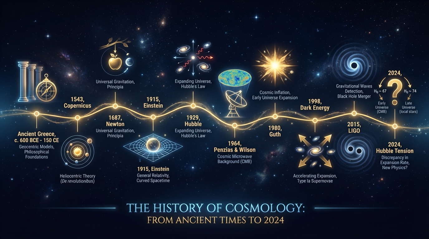
Figure 0.1: Historical Development of Cosmology
0.1 From Myths to Science: Ancient Period to Newton
Briefly: In ancient Greece, Aristotle (384-322 BC) conceived a cosmos where Earth was at the center and celestial bodies moved in perfect circular orbits.
From the moment humanity first looked at the sky, they wondered about the nature of the universe. In ancient Greece, Aristotle (384-322 BC) conceived a cosmos where Earth was at the center and celestial bodies moved in perfect circular orbits. Ptolemy (100-170 AD) mathematically developed this geocentric model — and it was accepted for 1400 years.
The Copernican Revolution (1543): Nicolaus Copernicus placed the Sun at the center in his work "De revolutionibus orbium coelestium." This radical idea began to question humanity's place in the universe. Galileo Galilei (1610) confirmed Copernicus by observing Jupiter's moons with his telescope — and faced the wrath of the Inquisition.
Newton's Synthesis (1687): Isaac Newton presented the universal law of gravitation in his "Philosophiæ Naturalis Principia Mathematica":
Showing that the same law that makes an apple fall also keeps the Moon in orbit was a scientific revolution. The universe now worked like a mechanical clock — deterministic, predictable, infinite.
0.2 The Einstein Revolution: Discovery of Spacetime Fabric (1905-1929)
Briefly: One of them was the Special Theory of Relativity: Time and space are not absolute, but relative!
1905: Annus Mirabilis - Albert Einstein, a 26‑year‑old patent clerk, published 4 papers that fundamentally changed physics. One of them was the Special Theory of Relativity: Time and space are not absolute, but relative!
1915: General Relativity - Einstein redefined gravitation. It was no longer a "force," but the curvature of spacetime:
"Matter tells spacetime how to curve; spacetime tells matter how to move." - John Archibald Wheeler
Einstein's "Greatest Mistake": In 1917, Einstein believed the universe was static. He added a cosmological constant (Λ) to balance his equations. After Hubble discovered the expanding universe in 1929, he called it "the biggest blunder of my life."
Ironically, with the discovery of dark energy in 1998, Λ returned — perhaps Einstein's greatest "mistake" was actually his deepest insight!
Friedmann & Lemaître: The Expanding Universe
In 1922, Russian mathematician Alexander Friedmann showed that Einstein's equations have solutions for an expanding or contracting universe. Einstein initially rejected it (1922 letter: "Your calculations are correct but have no physical meaning"), then admitted his mistake in 1923.
In 1927, Belgian priest‑physicist Georges Lemaître independently reached the same conclusion and proposed the "primeval atom" idea — the first version of the Big Bang! Einstein's comment: "Your calculations are correct, but your physics is abominable."
0.3 Hubble's Discovery: The Universe is Expanding! (1929)
Briefly: In 1929, he made a revolutionary discovery: Galaxies are moving away from us, and the farther they are, the faster they move!
Edwin Hubble observed galaxies with the 100‑inch telescope at Mount Wilson Observatory. In 1929, he made a revolutionary discovery: Galaxies are moving away from us, and the farther they are, the faster they move!
This simple relation was direct evidence that the universe is expanding. If galaxies are moving apart, they must have been closer in the past — even at a single "atom" at one point!
The Term "Big Bang": Ironically, Fred Hoyle (1949) was the first to use this term — and he used it mockingly! Hoyle was a proponent of the Steady State theory and opposed the idea that the universe had a beginning. But the term stuck and became the popular name for the Big Bang theory.
0.4 Golden Age Discoveries: CMB, Dark Matter, Inflation (1960-2000)
Briefly: Gives a concise explanation of CMB, Dark Matter, Inflation.
1964: Accidental Discovery - Cosmic Microwave Background
Briefly: There was a mysterious "noise" — from all directions, at all times.
Arno Penzias and Robert Wilson were testing a new radio antenna at Bell Labs. There was a mysterious "noise" — from all directions, at all times. They cleaned the pigeon droppings inside the antenna. The noise continued!
Nearby at Princeton, Robert Dicke's team was searching for the "afterglow" of the Big Bang. The two groups came together: Penzias & Wilson had unknowingly discovered Cosmic Microwave Background (CMB) radiation — at 3K, exactly as George Gamow had predicted in 1948!
Nobel Prize (1978) - The strongest evidence for the Big Bang theory.
1970s: Vera Rubin and Dark Matter
Briefly: But she continued observing galaxy rotation curves.
Vera Rubin, as a female astronomer, faced many challenges in the 1960s. But she continued observing galaxy rotation curves. The result was shocking: Stars were rotating much faster than the gravity of visible matter could account for!
In 1933, Fritz Zwicky had used the term "dunkle Materie" (dark matter), but it was ignored for 40 years. Rubin's systematic observations were now undeniable: 85% of the universe is invisible!
1980: Alan Guth's Eureka Moment - Inflation
Briefly: Late at night, he scribbled in his notebook: "SPECTACULAR REALIZATION!".
In 1979, young physicist Alan Guth at Stanford was thinking about the magnetic monopole problem. Late at night, he scribbled in his notebook: "SPECTACULAR REALIZATION!"
If the universe underwent exponential expansion (inflation) in the first 10⁻³⁵ seconds, the horizon problem, flatness problem, and monopole problem would all be solved simultaneously! Inflation theory was born.
1998: The Dark Energy Shock
Briefly: Expectation: The universe is slowing down.
Two independent teams (Supernova Cosmology Project - Saul Perlmutter, High-Z Team - Brian Schmidt & Adam Riess) observed distant supernovae. Expectation: The universe is slowing down. Result: The universe is accelerating!
Saul Perlmutter: "My first reaction: We made a mistake. My second: Did the rival team make the same mistake? My third: Everything we know about the universe is wrong!"
Dark energy was discovered — 68% of the universe. Nobel Prize (2011).
0.5 21st Century: Precision Cosmology and New Crises
Briefly: Gives a concise explanation of Precision Cosmology and New Crises.
2003-2013: WMAP and Planck - CMB Maps
Briefly: Result: ΛCDM model fits perfectly!
WMAP (Wilkinson Microwave Anisotropy Probe) and Planck satellites mapped the CMB with extraordinary precision. Result: ΛCDM model fits perfectly! Cosmological parameters determined with 1% accuracy.
2015: LIGO - Gravitational Waves
Briefly: The waves predicted by Einstein 100 years ago were finally found!
September 14, 2015, 09:50:45 UTC: LIGO detectors detected gravitational waves from the merger of two black holes 1.3 billion light years away. The waves predicted by Einstein 100 years ago were finally found!
Nobel Prize (2017) - A new observational window opened.
2014: The BICEP2 Drama
Briefly: Direct evidence for inflation theory!
The BICEP2 team announced they had detected the B‑mode signal of primordial gravitational waves. Direct evidence for inflation theory! The media went wild.
But Planck data showed: The signal came from galactic dust. BICEP2 retracted. The importance of the scientific process: The error correction mechanism worked.
2019-2025: Hubble Tension - The Crisis Deepens
Briefly: The probability of being a "fluke" is less than one in a million.
Early universe (Planck CMB): H₀ = 67.4 km/s/Mpc
Late universe (SH0ES 2024/2025): H₀ = 73.04 km/s/Mpc
6σ tension! The probability of being a "fluke" is less than one in a million. DESI 2025 results, while consistent with ΛCDM, gave the first serious hints that dark energy may vary with time (w ≠ -1). Solutions: Roman Space Telescope (2027) and new physics...
Present (2024): Cosmology is in the era of "precision science." But new questions are emerging:
- Will the Hubble Tension be resolved?
- Will the dark matter particle be found?
- What is the nature of dark energy?
- Can quantum gravity be observed?
- Is the multiverse real?
The story of the universe continues — and the most exciting chapters have yet to be written!
Fundamental Concepts and the Geometry of the Universe
This chapter explains how the assumptions of homogeneity/isotropy translate into FLRW geometry and are tested by measurements. The aim is to establish a common conceptual language and geometric tools for the derivations in subsequent chapters.
"To grasp reality, one must understand the entire mechanism."
1.1 The Cosmological Principle: Homogeneity and Isotropy
Briefly: This principle assumes that on large scales (about 100 Mpc and above), the universe is both homogeneous (the same everywhere) and isotropic (the same in all directions).
The cornerstone of modern cosmology is the Cosmological Principle. This principle assumes that on large scales (about 100 Mpc and above), the universe is both homogeneous (the same everywhere) and isotropic (the same in all directions).
Historical Perspective
Briefly: The Cosmological Principle is a mathematical expression of this philosophical approach: There is no privileged position or direction in the universe.
With the Copernican revolution, humanity began to move away from its central position in the universe. The Cosmological Principle is a mathematical expression of this philosophical approach: There is no privileged position or direction in the universe.
Observational Support
Briefly: COBE, WMAP, and Planck satellites have proven that the CMB is isotropic to within 10⁻⁵.
Large Scale Structure observations (2dF, SDSS) show that the universe is homogeneous on scales of about 100 Mpc. COBE, WMAP, and Planck satellites have proven that the CMB is isotropic to within 10⁻⁵. The distance‑redshift relations of Type Ia supernovae in different directions are consistent.
Important Note: The Cosmological Principle is an approximation. On small scales (stars, galaxies, galaxy clusters), the universe is clearly not homogeneous. Statistical homogeneity only emerges on very large scales.
Mathematical Formulation
Briefly: If space is homogeneous and isotropic on a constant‑t surface, the metric must have a maximally symmetric form.
Homogeneity and isotropy impose strong constraints on the spacetime metric. If space is homogeneous and isotropic on a constant‑t surface, the metric must have a maximally symmetric form.
Isotropy Condition: All directions are equivalent for an observer.
Homogeneity Condition: All spatial points are equivalent (no preferred center).
Dipole Anisotropy and Observer Motion
Briefly: This dipole allows us to measure our velocity relative to the cosmic reference frame.
The CMB dipole is not a physical structure that breaks the large‑scale isotropy of the universe, but a Doppler effect due to the observer's motion. This dipole allows us to measure our velocity relative to the cosmic reference frame.
Ehlers–Geren–Sachs (EGS) Theorem
Briefly: This theorem strengthens the mathematical foundation of the cosmological principle.
The EGS theorem shows that under sufficient observational conditions, isotropy forces homogeneity. This theorem strengthens the mathematical foundation of the cosmological principle.
Statistical Cosmological Principle
Briefly: Therefore, "statistical" homogeneity is accepted, not "exact" homogeneity.
The fact that the universe is homogeneous and isotropic on large scales does not contradict local structure. Therefore, "statistical" homogeneity is accepted, not "exact" homogeneity.
Correlation Function
Briefly: The two‑point correlation function is used to statistically measure the distribution of matter.
The two‑point correlation function is used to statistically measure the distribution of matter:
The Copernican Principle
Briefly: The assumption that the universe grants no special privilege to any observer forms the philosophical foundation of modern cosmology.
The assumption that the universe grants no special privilege to any observer forms the philosophical foundation of modern cosmology.
Bianchi Classifications and the FLRW Limit
Briefly: FLRW is the isotropic limit of these classes and carries maximal symmetry.
Homogeneous 3‑manifolds are categorized by Bianchi classes. FLRW is the isotropic limit of these classes and carries maximal symmetry.
1.2 General Relativity and Gravitation
Briefly: Gives a concise explanation of General Relativity and Gravitation.
Einstein's Revolutionary Theory
Briefly: Unlike Newton's instantaneous action theory, General Relativity predicts that gravitational interactions propagate at the speed of light.
In 1915, Albert Einstein formulated the General Theory of Relativity, which redefined gravitation as the curvature of spacetime. Unlike Newton's instantaneous action theory, General Relativity predicts that gravitational interactions propagate at the speed of light.
Einstein Field Equations
Briefly: "Matter tells spacetime how to curve; curved spacetime tells matter how to move" - John Archibald Wheeler.
The heart of General Relativity is the Einstein Field Equations:
Where:
- Gμν: Einstein tensor (describes spacetime curvature)
- gμν: Metric tensor (describes spacetime geometry)
- Λ: Cosmological constant
- G: Newton's gravitational constant
- c: Speed of light
- Tμν: Energy‑momentum tensor
"Matter tells spacetime how to curve; curved spacetime tells matter how to move" - John Archibald Wheeler
Cosmological Constant: Λ
Briefly: After Hubble discovered the expanding universe, Einstein called it his "greatest mistake." Ironically, with the discovery of dark energy in the 1990s, Λ returned to cosmology.
Einstein initially added the cosmological constant to obtain a static universe. After Hubble discovered the expanding universe, Einstein called it his "greatest mistake." Ironically, with the discovery of dark energy in the 1990s, Λ returned to cosmology.
Newtonian Limit and Transition to Cosmology
Briefly: This approximation allows an intuitive derivation of the Friedmann equations.
In the weak field and low velocity limit, General Relativity reduces to the Newtonian potential. This approximation allows an intuitive derivation of the Friedmann equations. For the small potential limit:
This limit relates the expansion dynamics of the universe to Newtonian energy conservation, combining geometric interpretation with physical intuition.
Energy‑Momentum Tensor and Perfect Fluid
Briefly: Here ρ is energy density, p is pressure, and u is the four‑velocity of the fluid.
In cosmology, matter content is mostly modeled as a perfect fluid. In this case:
Here ρ is energy density, p is pressure, and u is the four‑velocity of the fluid. This form clearly shows the gravitational role of pressure in the dynamics of the universe.
Variational Principle and Derivation of Field Equations
Briefly: The Einstein‑Hilbert action.
Einstein's equations are derived from the action principle. The Einstein‑Hilbert action:
This formulation ensures the mathematical consistency of symmetry assumptions used in cosmological models and opens the door to discussions of quantum gravity.
Energy Conditions and Physical Limits
Briefly: Violations of these conditions give rise to the fundamental physical discussions of accelerated expansion regimes such as dark energy and inflation.
Within General Relativity, energy conditions constrain physically reasonable types of matter:
- NEC: ρ + p/c² ≥ 0
- WEC: ρ ≥ 0 and ρ + p/c² ≥ 0
- SEC: ρ + 3p/c² ≥ 0
Violations of these conditions give rise to the fundamental physical discussions of accelerated expansion regimes such as dark energy and inflation.
1.3 The FLRW Metric: The Measure of Spacetime
Briefly: In 1922, Russian mathematician Alexander Friedmann showed that Einstein's field equations have solutions for an expanding or contracting universe.
Historical Perspective: Friedmann's Struggle
In 1922, Russian mathematician Alexander Friedmann showed that Einstein's field equations have solutions for an expanding or contracting universe. He wrote a letter to Einstein.
Einstein's first response (1922): "Your calculations are correct but have no physical meaning. The universe is static." Einstein rejected Friedmann's work.
1923: Einstein realized his mistake and published a correction in Zeitschrift für Physik: "In my previous note, Mr. Friedmann's results are correct and shed new light."
Unfortunately, Friedmann died of typhoid in 1925 at the age of 37 — without seeing the observational evidence for the expanding universe (Hubble, 1929).
The Friedmann‑Lemaître‑Robertson‑Walker Metric
Briefly: Figure 1.1: Geometry of the Universe: Open (k=-1), Flat (k=0), and Closed (k=+1) Models.
Applying the Cosmological Principle, the spacetime geometry of the universe is uniquely described by the FLRW metric.
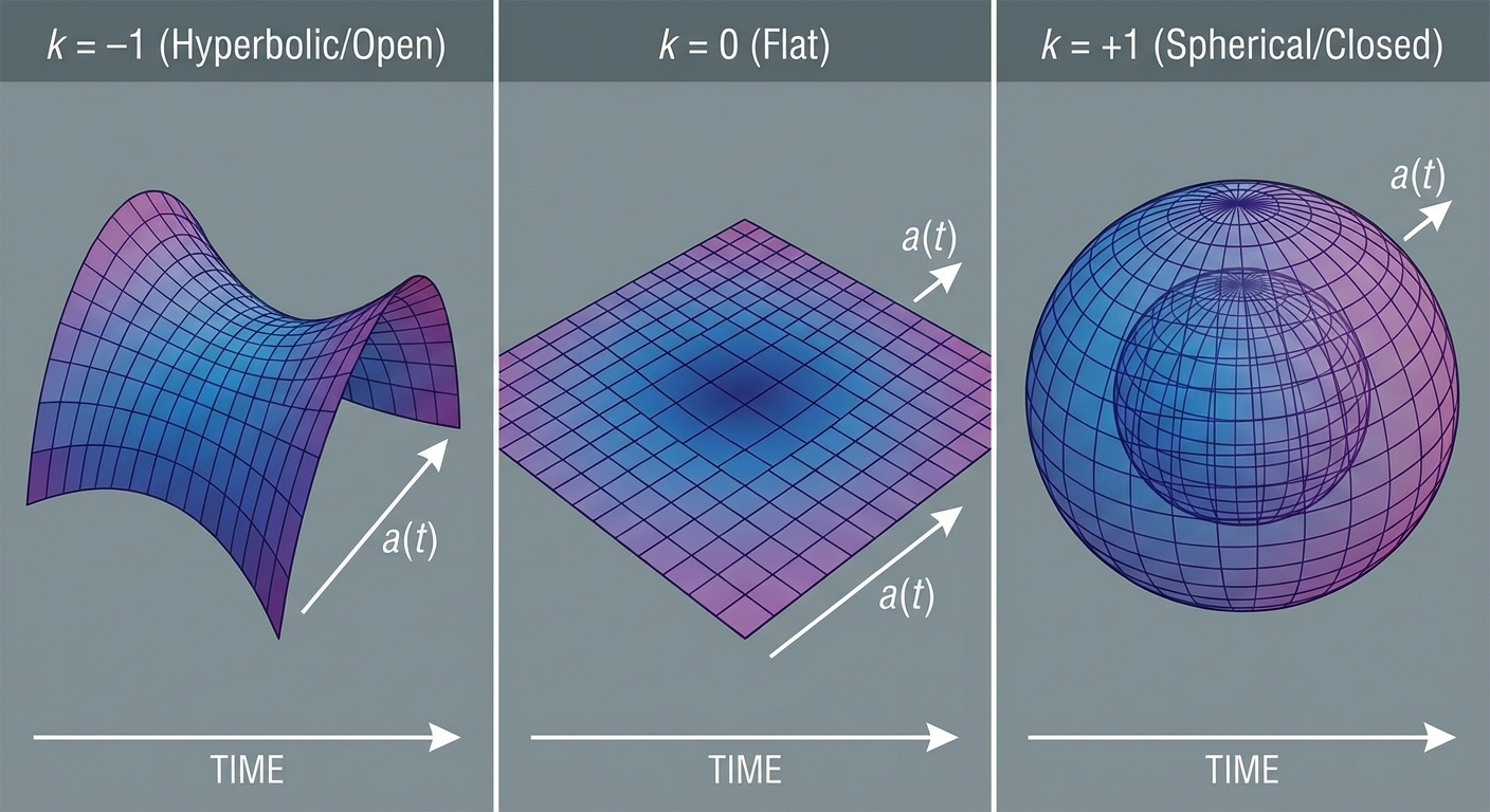
Figure 1.1: Geometry of the Universe: Open (k=-1), Flat (k=0), and Closed (k=+1) Models
Scale Factor: a(t)
Briefly: It is usually normalized so that a(t₀) = 1 (today).
The scale factor a(t) is a function of time that describes the expansion or contraction of the universe. It is usually normalized so that a(t₀) = 1 (today). The physical distance between two comoving points is:
Curvature Parameter: k
Briefly: Current Observations: Planck satellite data (2018) confirm the flatness of the universe with extraordinary precision: Ωtotal = 0.9993 ± 0.0019.
The parameter k describes the geometric curvature of space and can take three values:
- k = 0: Flat (Euclidean) space — Parallel lines never meet
- k = +1: Closed (spherical) space — Positive curvature, finite volume
- k = -1: Open (hyperbolic) space — Negative curvature, infinite space
Current Observations: Planck satellite data (2018) confirm the flatness of the universe with extraordinary precision: Ωtotal = 0.9993 ± 0.0019
Conformal Time (η)
Briefly: Conformal time rescales cosmic time to track light‑cone distances and horizons.
Conformal time is used to analyze the journey of light and cosmic horizons:
This definition clarifies the geometric origins of the horizon problem and plays a fundamental role in CMB analysis.
Hubble Parameter and Hubble Scale
Briefly: H(t) gives the expansion rate; c/H sets the characteristic horizon scale.
The expansion rate is defined by H(t):
The Hubble scale L_H gives the characteristic length scale of universal dynamics.
Observational Distance Definitions
Briefly: This relation is known as Etherington's reciprocity relation and is a fundamental consistency test in modern cosmology.
Different distance definitions are used in cosmology, each corresponding to different observations:
- Comoving distance: coordinate distance not scaled by expansion
- Proper distance: physical distance
- Luminosity distance: distance used in brightness measurements
- Angular diameter distance: distance used in angular size measurements
This relation is known as Etherington's reciprocity relation and is a fundamental consistency test in modern cosmology.
Introduction to Perturbation Theory
Briefly: Small deviations are necessary for the formation of cosmic structures.
The real universe is not perfectly homogeneous. Small deviations are necessary for the formation of cosmic structures:
These small perturbations are decomposed into scalar, vector, and tensor modes and explain the origin of cosmological structures.
Friedmann Equations and the Dynamics of the Universe
This chapter establishes the Friedmann equations that determine the expansion dynamics of the universe and the role of energy contents in this dynamics. The aim is to connect the physical meaning of the Hubble evolution and density parameters directly to observational quantities.
"When trying to explain nature, we have a wonderful method called science."
2.1 The First Friedmann Equation: Expansion Rate Analysis
Briefly: In 1927, Belgian priest‑physicist Georges Lemaître independently found the expanding universe solution and proposed the "primeval atom" idea — the first version of the Big Bang!
Historical Perspective: Lemaître's Foresight
In 1927, Belgian priest‑physicist Georges Lemaître independently found the expanding universe solution and proposed the "primeval atom" idea — the first version of the Big Bang!
Einstein's reaction: "Your calculations are correct, but your physics is abominable."
Ironic fact: Lemaître mathematically showed that the universe was expanding 2 years before Hubble (1927 vs 1929)! But his paper was published in French and was overlooked.
In 1931, Lemaître published an English paper in Nature. It could no longer be ignored. Einstein finally admitted: "This is the most beautiful and satisfying explanation of cosmology."
Applying the Einstein Field Equations to the FLRW metric yields the Friedmann Equations that govern the dynamics of the universe.
Where:
- H(t) = ȧ/a: Hubble parameter (expansion rate)
- ρ: Total energy density
- k: Curvature parameter (-1, 0, +1)
- Λ: Cosmological constant
Derivation from GR
Briefly: This component relates spacetime curvature to the energy density of the universe, directly determining the expansion dynamics.
The 00 component of the Einstein equations is taken for the FLRW metric. This component relates spacetime curvature to the energy density of the universe, directly determining the expansion dynamics. In summary:
This expression, combined with T^0{}_0 = -\rho c^2, gives the Friedmann equation.
Newtonian Derivation
Briefly: Choosing R = a(t) r gives the Newtonian version of the Friedmann equation, where the energy term corresponds to the curvature parameter.
Energy conservation for a test particle under spherical symmetry gives:
Choosing R = a(t) r gives the Newtonian version of the Friedmann equation, where the energy term corresponds to the curvature parameter.
Density Parameters
Briefly: These definitions allow quantitative tracking of the geometry of the universe and how components become dominant over time.
Cosmological density parameters are defined as:
These definitions allow quantitative tracking of the geometry of the universe and how components become dominant over time.
Physical Interpretation
Briefly: This equation shows that the expansion rate of the universe depends on three factors: the Matter/Energy term creates gravitational attraction, the Curvature term has a geometric effect, and the Cosmological Constant term has a "repulsive" effect.
This equation shows that the expansion rate of the universe depends on three factors: the Matter/Energy term creates gravitational attraction, the Curvature term has a geometric effect, and the Cosmological Constant term has a "repulsive" effect.
Critical Density
Briefly: Its current value is approximately 1.88 × 10⁻²⁹ h² g/cm³ ≈ 10⁻²⁶ kg/m³.
Critical density is the density required for a flat universe (k=0):
Its current value is approximately 1.88 × 10⁻²⁹ h² g/cm³ ≈ 10⁻²⁶ kg/m³.
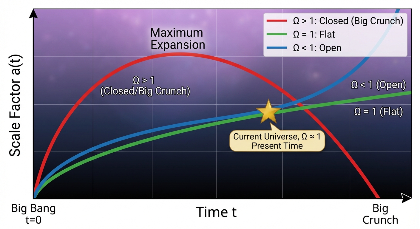
Figure 2.1: Future of the Universe According to the Density Parameter (Ω)
Current Values (Planck 2018)
Briefly: The Planck satellite has determined cosmological parameters with extraordinary precision through CMB observations.
The Planck satellite has determined cosmological parameters with extraordinary precision through CMB observations:
- Ωm,0 ≈ 0.315 (Total matter)
- ΩΛ,0 ≈ 0.685 (Dark energy)
- Ωr,0 ≈ 9 × 10⁻⁵ (Radiation)
- Ωk,0 ≈ 0.001 ± 0.002 (Nearly zero - flat universe)
2.2 The Second Friedmann Equation: Acceleration and the Effect of Pressure
Briefly: The first term shows the gravitational decelerating effect of matter and energy.
This equation describes the acceleration of the universe. The first term shows the gravitational decelerating effect of matter and energy. Pressure also has a gravitational effect — this is an important difference between General Relativity and Newtonian theory.
The 1998 Discovery: Teams led by Saul Perlmutter, Brian Schmidt, and Adam Riess discovered that the universe is accelerating by observing distant Type Ia supernovae (Nobel Prize, 2011). This unexpected result is the strongest evidence for the existence of dark energy.
Acceleration with Equation of State
Briefly: The condition for acceleration is w < -1/3, which requires dark energy to have negative pressure.
The w parameter, the ratio of pressure to density, determines the acceleration condition:
The condition for acceleration is w < -1/3, which requires dark energy to have negative pressure.
Raychaudhuri Perspective
Briefly: This shows that expansion evolves into contraction or expansion regimes depending on energy conditions.
The acceleration equation is the isotropic limit of the Raychaudhuri equation. This shows that expansion evolves into contraction or expansion regimes depending on energy conditions.
Deceleration vs Acceleration
Briefly: Accelerating Universe (ä > 0): Condition: ρ + 3p/c² < Λc²/(4πG) - Dark energy dominated era (today!).
Decelerating Universe (ä < 0): Condition: ρ + 3p/c² > Λc²/(4πG) - Matter or radiation dominated eras
Accelerating Universe (ä > 0): Condition: ρ + 3p/c² < Λc²/(4πG) - Dark energy dominated era (today!)
2.3 Contents of the Universe: Equation of State Parameter (w)
Briefly: Here w is the dimensionless equation of state parameter.
An equation of state is defined for each cosmic component:
Here w is the dimensionless equation of state parameter:
- Dust (w = 0): Cold matter, pressure negligible, $$\rho_m \propto a^{-3}$$
- Radiation (w = 1/3): Photons, neutrinos, $$\rho_r \propto a^{-4}$$
- Cosmological Constant (w = -1): Dark energy, $$\rho_\Lambda = \text{constant}$$
Continuity Equation
Briefly: This equation determines how different components dilute or remain constant over time.
Energy conservation reduces to a continuity equation specific to cosmology:
This equation determines how different components dilute or remain constant over time.
Acceleration Condition: From the second Friedmann equation, acceleration requires w < -1/3. Therefore, matter and radiation decelerate, while dark energy accelerates.
2.4 Critical Density and Density Parameter (Ω)
Briefly: The total density parameter Ωtotal determines the geometry and ultimate fate of the universe.
The total density parameter Ωtotal determines the geometry and ultimate fate of the universe:
- Ωtotal > 1 (k = +1): Closed universe, will eventually collapse
- Ωtotal = 1 (k = 0): Flat universe, expands forever
- Ωtotal < 1 (k = -1): Open universe, expands forever
The Flatness Problem
Briefly: This is not a coincidence — it creates a fine‑tuning problem for the early universe.
Observations show the universe is remarkably flat (Ωtotal ≈ 1). This is not a coincidence — it creates a fine‑tuning problem for the early universe. For Ωtotal ≈ 1 today, |Ω - 1|Planck < 10⁻⁶⁰ must hold at Planck time. This extraordinary fine‑tuning is one of the motivations for inflation theory.
Curvature and Observational Constraints
Briefly: Modern data confirm the flatness of the universe at the 0.2% level.
Strong constraints on the curvature parameter are obtained by combining BAO, CMB acoustic peak positions, and lensing measurements. Modern data confirm the flatness of the universe at the 0.2% level.
The Cosmological Standard Model (ΛCDM)
This chapter shows the components of ΛCDM and how they are tested by CMB/LSS. The aim is to clarify the observational bases of the components that make up the "cosmic budget" and the limits of the model.
"Facts demand a simple explanation within the big picture of complexity."
3.1 The Cosmic Budget: Matter, Radiation, and Dark Energy
Briefly: This model describes the content of the universe with three main components.
ΛCDM (Lambda‑Cold Dark Matter) is the standard model of cosmology. This model describes the content of the universe with three main components:
- Dark Energy (Λ): ~68.5%
- Cold Dark Matter (CDM): ~26.6%
- Baryonic Matter: ~4.9%
- Radiation (photons + neutrinos): ~0.01%
Planck 2018 Results:
- H₀ = 67.4 ± 0.5 km/s/Mpc
- Ωb h² = 0.02237 ± 0.00015
- Ωc h² = 0.1200 ± 0.0012
- ΩΛ = 0.6847 ± 0.0073
Dark Matter
Briefly: It is non‑relativistic and plays a critical role in structure formation.
Cold Dark Matter does not emit or absorb electromagnetic radiation and interacts only through gravity. It is non‑relativistic and plays a critical role in structure formation.
Dark Energy
Briefly: It has negative pressure (w ≈ -1), and its physical nature is one of the deepest mysteries of modern physics.
Dark energy is the mysterious form of energy responsible for the accelerated expansion of the universe. It has negative pressure (w ≈ -1), and its physical nature is one of the deepest mysteries of modern physics.
3.2 Thermal History of the Universe: Eras of Dominance
Briefly: The history of the universe is divided into eras based on which component dominates the energy density.
The history of the universe is divided into eras based on which component dominates the energy density:
Planck Era (t < 10⁻⁴³ s)
Quantum gravity effects are dominant. Classical spacetime concepts are invalid. Planck temperature: TP ≈ 1.4 × 10³² K
Grand Unified Era (10⁻⁴³ s < t < 10⁻³⁶ s)
The strong and electroweak forces are unified. Inflation likely occurs during this period.
Nucleosynthesis (3 minutes < t < 20 minutes)
Light elements are synthesized: D, ³He, ⁴He, ⁷Li. Helium‑4 abundance: Yp ≈ 0.25
Recombination (t ~ 380,000 years)
Briefly: The universe becomes transparent, and CMB photons begin to travel freely.
Electrons combine with protons to form neutral hydrogen atoms. The universe becomes transparent, and CMB photons begin to travel freely.
Dark Energy Dominance (z < 0.5)
For the last ~5 billion years, dark energy has surpassed matter. The universe has begun to accelerate.
3.3 Cosmic Microwave Background (CMB): The First Light
Briefly: Gives a concise explanation of The First Light.
Discovery of the CMB
Briefly: This discovery became the strongest confirmation of the Big Bang theory.
In 1964, Arno Penzias and Robert Wilson accidentally discovered cosmic microwave background radiation (Nobel Prize, 1978). This discovery became the strongest confirmation of the Big Bang theory.
Historical Perspective: Accidental Discovery - Penzias & Wilson
In 1964, Arno Penzias and Robert Wilson were testing a new radio antenna at Bell Labs. There was a mysterious "noise" — from all directions, at all times, at a temperature of 3.5K.
Their first thoughts: It must be a technical problem. Radio noise from New York City? Pigeon droppings inside the antenna? They cleaned the antenna and chased away the pigeons. The noise continued!
Nearby at Princeton, Robert Dicke's team was searching for the "afterglow" of the Big Bang. The two groups came together: Penzias & Wilson had unknowingly discovered Cosmic Microwave Background (CMB) radiation!
Ironic detail: George Gamow and his students (Ralph Alpher & Robert Herman) had predicted the CMB in 1948 (~5K). But no one looked for it. It was found by accident 16 years later!
Nobel Prize (1978) - The strongest evidence for the Big Bang theory. Dicke's comment: "They scooped us!"
The CMB consists of photons from the recombination era (z ~ 1100, t ~ 380,000 years). At that time, T ~ 3000 K; today, T = 2.7255 ± 0.0006 K.
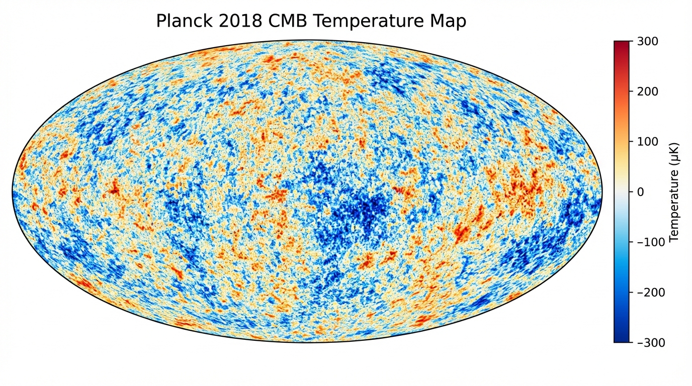
Figure 3.1: Planck Satellite CMB Temperature Map (2018)
Anisotropies: The CMB is almost perfectly isotropic, but there are small temperature fluctuations: ΔT/T ~ 10⁻⁵. These fluctuations reflect density fluctuations in the early universe and are the seeds of today's structures.
COBE, WMAP, and Planck
Briefly: WMAP (2001-2010): Determined cosmological parameters with 1% accuracy.
COBE (1989-1993): Confirmed the blackbody spectrum of the CMB
WMAP (2001-2010): Determined cosmological parameters with 1% accuracy
Planck (2009-2013): Most precise CMB map, determined cosmological parameters with 0.5% accuracy
3.4 BBN: Big Bang Nucleosynthesis
Briefly: It (BBN) is the synthesis of light elements that occurred 3‑20 minutes after the Big Bang.
Big Bang Nucleosynthesis (BBN) is the synthesis of light elements that occurred 3‑20 minutes after the Big Bang.
Synthesized Elements
Briefly: Obtaining the same result from independent epochs is strong confirmation of the Big Bang model.
- Deuterium (D): D/H ~ 2.5 × 10⁻⁵
- Helium-4: Yp ≈ 0.25 (by mass)
- Helium-3: ³He/H ~ 10⁻⁵
- Lithium-7: ⁷Li/H ~ 10⁻¹⁰
BBN and CMB Consistency: The baryon density determined from BBN (Ωb h² = 0.0224 ± 0.0001) and from CMB (0.02237 ± 0.00015) show remarkable agreement. Obtaining the same result from independent epochs is strong confirmation of the Big Bang model.
3.5 Neutrino Cosmology and Neff
Neutrinos decouple from thermal equilibrium in the early universe and stream freely, suppressing structure formation. Their effects are typically parameterized by the effective number of species $$N_{\text{eff}}$$ and the total mass $$\sum m_\nu$$.
The Standard Model expects $$N_{\text{eff}} \approx 3.046$$. Additional relativistic species are strongly constrained by CMB and BBN.
Neutrino masses suppress the power spectrum on small scales and provide tight constraints when combined with $$\sigma_8$$ measurements.
Cosmic Neutrino Background (CNB)
Briefly: The CNB is the relic neutrino background, inferred indirectly through its imprint on the CMB and large‑scale structure.
The CNB is the neutrino counterpart of the CMB, with today's $$T_\nu \approx 1.95\,\text{K}$$. Although direct detection is difficult, its effects are indirectly measured through CMB and LSS.
Mass Hierarchy
Briefly: Mass hierarchy refers to the ordering of neutrino masses and affects the summed mass and growth suppression.
The normal and inverted hierarchies are tested through the total mass $$\sum m_\nu$$ and the suppression of growth. Future CMB‑S4 and LSS surveys aim to distinguish them.
Decoupling and Free‑Streaming
Briefly: Decoupling ends neutrino interactions, while free‑streaming damps small‑scale structure.
Neutrinos decouple from thermal equilibrium when the weak interaction rate drops below the expansion rate:
The free‑streaming length suppresses small‑scale density fluctuations and produces a scale‑dependent break in the power spectrum.
3.6 CMB Anisotropy Formalism (SW/ISW/Doppler)
Briefly: This decomposition shows that different physical processes dominate in the low‑ℓ and high‑ℓ regions.
CMB temperature anisotropies are explained by three main components:
- Sachs–Wolfe (SW): Redshift from potential wells
- Integrated SW: Integral of time‑varying potentials
- Doppler: Velocity field of the photon‑baryon fluid
This decomposition shows that different physical processes dominate in the low‑ℓ and high‑ℓ regions.
Power Spectrum and Line‑of‑Sight Approach
Briefly: The line‑of‑sight integral is a standard technique in CAMB/CLASS to efficiently solve the Boltzmann hierarchy.
The CMB power spectrum $$C_\ell$$ is the convolution of the primordial spectrum with transfer functions:
The line‑of‑sight integral is a standard technique in CAMB/CLASS to efficiently solve the Boltzmann hierarchy.
The transfer function $$\Delta_\ell(k)$$ is the projection of the source function onto spherical Bessel functions:
This formula unifies the sources of temperature and polarization anisotropies (SW, ISW, Doppler, lensing) under a single framework.
The source function $$S(k,\eta)$$ is weighted by the visibility function $$g(\eta) = \dot{\tau} e^{-\tau}$$, so that the thickness of the last scattering surface and late‑time contributions are collected in the same integral form.
ISW Term (Explicit Form)
Briefly: The late‑time ISW becomes important during the dark energy era and is measured through correlation with LSS.
Time‑varying potentials contribute to the integrated Sachs‑Wolfe effect:
The late‑time ISW becomes important during the dark energy era and is measured through correlation with LSS.
Boltzmann Hierarchy (Summary)
Briefly: CAMB/CLASS numerically solve this hierarchy.
The multipole moments of the photon distribution evolve with a hierarchy that includes collision and free‑streaming terms. CAMB/CLASS numerically solve this hierarchy.
3.7 Large Scale Structure (LSS) and Halo Model
Briefly: Beyond the linear regime, the halo model provides a statistical description of large‑scale structure.
Linear growth is described by the perturbation equation:
Beyond the linear regime, the halo model provides a statistical description of large‑scale structure.
Press–Schechter Approach
Briefly: Here $$\delta_c \approx 1.686$$ is the spherical collapse threshold.
The halo mass function is based on the probability of regions collapsing above a critical threshold.
Here $$\delta_c \approx 1.686$$ is the spherical collapse threshold. Modern studies use Sheth–Tormen corrections to account for elliptical collapse effects.
Bias and RSD
Briefly: Galaxy‑matter bias and redshift‑space distortions are used to measure the velocity field and growth rate.
Galaxy‑matter bias and redshift‑space distortions are used to measure the velocity field and growth rate.
Halo Occupation Distribution (HOD)
Briefly: The HOD approach describes the statistical placement of galaxies in halos as a function of halo mass and is used to model the observed clustering signal.
The HOD approach describes the statistical placement of galaxies in halos as a function of halo mass and is used to model the observed clustering signal.
Non‑linear P(k)
Briefly: Halofit‑type recipes model the small‑scale behavior of $$P(k)$$.
In the non‑linear regime, perturbation theory and N‑body simulations are combined. Halofit‑type recipes model the small‑scale behavior of $$P(k)$$.
Non‑linear PT (2nd Order)
Briefly: This expression forms the basis for the bispectrum and non‑Gaussian structures.
The density contrast can be expanded with a second‑order kernel:
This expression forms the basis for the bispectrum and non‑Gaussian structures.
3.8 Cosmic Topology and Global Geometry Tests
Briefly: Multiply‑connected spaces would leave "circles‑in‑the‑sky" signatures in CMB maps.
The global topology of the universe can be directly tested by observations. Multiply‑connected spaces would leave "circles‑in‑the‑sky" signatures in CMB maps.
Topological tests, beyond the constraints on $$\Omega_k$$ and spatial curvature, provide a complementary tool to understand the global structure of the universe.
The "circles‑in‑the‑sky" method expects the same physical region in a multiply‑connected space to produce circular matches in the CMB. No strong matches have been found to date.
3.9 Modified Gravity and Alternative Theories
Briefly: These theories involve modifications of General Relativity on cosmological and galactic scales.
Since the nature of dark matter and dark energy remains unclear, some physicists have proposed alternative theories of gravity that do not require these invisible components. These theories involve modifications of General Relativity on cosmological and galactic scales.
Historical Development
Briefly: They replaced Newton's constant G with a dynamical scalar field.
1961 - Brans‑Dicke Theory: Carl Brans and Robert Dicke proposed the first serious generalization of General Relativity to incorporate Mach's principle into gravity. They replaced Newton's constant G with a dynamical scalar field.
1974 - Horndeski Theory: Gregory Horndeski formulated the most general scalar‑tensor theory yielding second‑order field equations. This work was largely forgotten until its rediscovery in the 2010s.
1980 - Starobinsky Inflation: Alexei Starobinsky proposed the f(R) = R + R²/(6M²) model. This could explain both early‑universe inflation and late‑time acceleration.
1983 - The MOND Revolution: Mordehai Milgrom proposed modifying Newtonian dynamics to explain galaxy rotation curves without dark matter. A radical alternative to the dark matter paradigm.
1998 - Discovery of Cosmic Acceleration: Supernova observations showed the universe is accelerating. This accelerated the search for dark energy or modified gravity.
2009 - Galileon Theories: Alberto Nicolis and colleagues developed scalar field theories with Galilean symmetry. They have the potential to explain cosmic acceleration through self‑acceleration mechanisms.
2010s - Horndeski Renaissance: Dark energy research rediscovered Horndeski's 1974 work. It became clear that Galileon, k‑essence, and other theories are all special cases of Horndeski theory.
2010s-2020s - Custon Fields: New theoretical frameworks combining curvature and tensor structures were developed. Efforts to explain dark matter and dark energy through geometric terms.
2017 - GW170817 Turning Point: Gravitational waves and electromagnetic signals from a neutron star merger were observed simultaneously. Result: cGW = c (with 10⁻¹⁵ precision). This excluded many modified gravity theories.
2018-2024 - Current Status: Precision observations from Planck, DES, and DESI continue to support ΛCDM. However, anomalies such as the Hubble tension and S8 tension keep modified gravity research active.
Paradigm Shifts: Theoretical curiosity in the 1960s, galaxy dynamics motivation in the 1980s, the 1998 discovery of cosmic acceleration, and tight constraints from GW170817 in 2017. Modified gravity theories have evolved with every major observational discovery in cosmology.
f(R) Gravity Theory
Briefly: Here f(R) is an arbitrary function of R.
f(R) theories replace the Ricci scalar R in the Einstein‑Hilbert action with a more general function f(R):
Here f(R) is an arbitrary function of R. General Relativity corresponds to the special case f(R) = R.
Starobinsky Model
Briefly: This model can explain cosmic acceleration without requiring dark energy.
The most successful f(R) model is Alexei Starobinsky's (1980) inflation model:
This model can explain cosmic acceleration without requiring dark energy. It is consistent with Planck 2018 data (ns = 0.965, r ≈ 0.003).
Observational Constraints: f(R) theories are constrained by Solar System tests (post‑Newtonian parameters), galaxy dynamics, and cosmological observations. Most simple f(R) models fail at least one of these tests.
Scalar‑Tensor Theories
Briefly: It replaces Newton's constant G with a dynamical scalar field φ.
Brans‑Dicke theory (1961) is the earliest generalization of General Relativity. It replaces Newton's constant G with a dynamical scalar field φ:
Here ωBD is the Brans‑Dicke parameter. Cassini spacecraft measurements: ωBD > 40,000.
Horndeski Theory
Briefly: It contains five free functions and avoids ghost instabilities.
The most general scalar‑tensor theory yielding second‑order field equations is Horndeski theory (1974). It contains five free functions and avoids ghost instabilities.
Custon Fields: Curvature‑Tensor Theories
Briefly: These theories aim to explain dark energy and dark matter through geometric terms.
Custon (curvature‑tensor) fields are a new theoretical framework that combines both curvature and tensor structures. These theories aim to explain dark energy and dark matter through geometric terms.
In custon theories, the action integral generally takes the form:
Here F is a general function that includes the Riemann tensor Rμνρσ, the Ricci tensor Rμν, the scalar curvature R, and derivatives of the custon field φ.
Properties of Custon Theories
Briefly: LIGO/Virgo gravitational wave observations and Euclid weak lensing data are critical for testing these theories.
- Geometric Dark Energy: Custon fields can produce effects similar to the cosmological constant but are dynamic
- Galaxy Rotation Curves: Some custon models can explain galaxy dynamics without dark matter
- Gravitational Lensing: Custon theories predict deviations from General Relativity in light deflection
- Gravitational Waves: The GW170817 observation (cGW = c) constrains many custon models
Current Status: Custon theories remain an active research topic. LIGO/Virgo gravitational wave observations and Euclid weak lensing data are critical for testing these theories.
MOND: Modified Newtonian Dynamics
Briefly: Here a₀ ≈ 1.2 × 10⁻¹⁰ m/s² is the critical acceleration, and μ(x) → 1 (x >> 1), μ(x) → x (x << 1).
Mordehai Milgrom (1983) proposed modifying Newton's second law instead of introducing dark matter:
Here a₀ ≈ 1.2 × 10⁻¹⁰ m/s² is the critical acceleration, and μ(x) → 1 (x >> 1), μ(x) → x (x << 1).
MOND's Successes:
- Explains galaxy rotation curves with a single parameter (a₀)
- Naturally predicts the Tully‑Fisher relation: $L \propto v^4$
- Successful for low surface brightness galaxies
MOND's Problems:
- Still requires dark matter in galaxy clusters
- Cannot explain CMB acoustic peak structure
- Inconsistent with Bullet Cluster observations
- Relativistic generalization (TeVeS) is complex and constrained
Galileon Models
Briefly: They explain cosmic acceleration through a self‑acceleration mechanism.
Galileon theories are scalar field theories with Galilean symmetry. They explain cosmic acceleration through a self‑acceleration mechanism:
Galileon fields can evade Solar System tests through the Vainshtein mechanism. However, the GW170817 observation has excluded many Galileon models.
Observational Tests and Constraints
Briefly: Conclusion: To date, no modified gravity theory has surpassed the success of General Relativity + dark matter + dark energy.
Modified gravity theories are constrained by multiple observational tests:
- Solar System: Post‑Newtonian parameters (γ, β) - Cassini: |γ-1| < 2.3×10⁻⁵
- Binary Pulsar: Periastron shift, orbital decay - PSR J0737-3039
- Gravitational Waves: GW170817: |cGW/c - 1| < 10⁻¹⁵
- Cosmology: CMB, BAO, SNe Ia, weak lensing - Planck + DES + BOSS
Conclusion: To date, no modified gravity theory has surpassed the success of General Relativity + dark matter + dark energy. However, research continues, and future observations (LISA, Einstein Telescope, Euclid) will provide more precise tests.
Inflation Theory and the Origin of Structure
This chapter explains how inflation solves the horizon/flatness problems and how quantum fluctuations are stretched to galactic scales. The aim is to clarify the testability of inflation through measurements of ns, r, and B‑modes.
"Humanity needs to see its intuitions on a cosmic scale."
4.1 Problems of the Traditional Model
Briefly: Gives a concise explanation of Problems of the Traditional Model.
Horizon Problem
Briefly: At the time of recombination, regions in different directions of the sky could never have been in causal contact.
Why do different directions of the CMB have the same temperature? At the time of recombination, regions in different directions of the sky could never have been in causal contact. So why is the entire sky at the same temperature (ΔT/T ~ 10⁻⁵)?
Expressed in conformal time, the causal influence region is:
At recombination, the horizon scale is much smaller than the angular separation we observe in the sky today, giving rise to the horizon problem.
Inflation solves this by exponentially expanding space over a short period, bringing regions that were previously in causal contact into view across large angles of the sky.
Flatness Problem
Briefly: Ω is unstable: any deviation from 1 grows exponentially.
Why is the universe so flat (Ωtotal ≈ 1)? Ω is unstable: any deviation from 1 grows exponentially. For Ωtotal = 1.000 ± 0.002 today, |Ω - 1|Planck < 10⁻⁶⁰ at Planck time. This extraordinary fine‑tuning requires an explanation.
Inflation suppresses the $$|\Omega-1|$$ term by growing $$a(t)$$ exponentially, making flatness a natural attractor.
Magnetic Monopole Problem
Briefly: These monopoles should dominate the universe today — but none have been observed.
Grand Unified Theories (GUTs) predict the production of heavy magnetic monopoles during symmetry breaking in the early universe. These monopoles should dominate the universe today — but none have been observed.
Entropy Problem and Initial Conditions
Briefly: While inflation explains the observed regularities through the exponential nature of expansion, the initial entropy problem remains controversial.
The universe starting with low entropy is an extraordinary special condition from a thermodynamic perspective. While inflation explains the observed regularities through the exponential nature of expansion, the initial entropy problem remains controversial. This issue is closely related to the Past Hypothesis and discussions of the cosmic arrow of time.
The entropy problem may require a more fundamental physics (e.g., quantum cosmology or multiverse) to explain initial conditions.
Horizon–Flatness–Homogeneity Common Structure
Briefly: Small deviations in phase space grow rapidly, making the standard Big Bang dynamics "fine‑tuned." Inflation suppresses this common sensitivity with an attractor dynamic.
These problems require extraordinarily precise selection of initial conditions. Small deviations in phase space grow rapidly, making the standard Big Bang dynamics "fine‑tuned." Inflation suppresses this common sensitivity with an attractor dynamic.
Historical Perspective: Guth's Eureka Moment
In 1979, young physicist Alan Guth at Stanford was thinking about the magnetic monopole problem. He worked late into the night. At midnight, an idea came...
He wrote in his notebook: "SPECTACULAR REALIZATION!"
If the universe had undergone exponential expansion (inflation) in the first 10⁻³⁵ seconds:
- The horizon problem is solved (causal contact is established)
- The flatness problem is solved (Ω → 1 is attracted)
- The monopole problem is solved (diluted)
Guth's comment (1997): "I had trouble sleeping that night. I was so excited. I checked the calculations the next day. They still worked!"
Inflation theory was born — and became one of the cornerstones of modern cosmology.
4.2 The Inflaton Field and Slow‑Roll Conditions
Briefly: Expansion factor: e⁶⁰⁻⁷⁰ ~ 10²⁶-10³⁰.
Alan Guth (1981) and Andrei Linde (1982) proposed inflation theory to solve these problems: an exponential expansion period in the very early universe.
Expansion factor: e⁶⁰⁻⁷⁰ ~ 10²⁶-10³⁰
Energy Density Composition (Inflaton)
Briefly: In the slow‑roll regime, potential energy dominates, giving $$w \approx -1$$ and enabling exponential expansion.
For the scalar inflaton field, energy density and pressure are:
In the slow‑roll regime, potential energy dominates, giving $$w \approx -1$$ and enabling exponential expansion.
This composition explains the "vacuum‑like" behavior of inflation and produces an expansion dynamic different from the classical matter/radiation regime.
Slow‑Roll Conditions
Briefly: Under slow‑roll conditions, the inflaton field slowly rolls down the potential, sustaining inflation.
A scalar field (φ, the inflaton) is assumed to drive inflation. Under slow‑roll conditions, the inflaton field slowly rolls down the potential, sustaining inflation.
Slow‑roll requires $$\epsilon \ll 1$$ and $$|\eta| \ll 1$$. These conditions give the effective equation of state $$w \approx -1$$ during inflation.
The slow‑roll parameters also determine the observed spectral index and tensor‑scalar ratio.
Potential Classes
Briefly: Gives a concise explanation of Potential Classes.
- Monomial: $$V(\phi) \propto \phi^p$$ (large field; most are observationally excluded)
- Plateau: Starobinsky, Higgs, α‑attractor (consistent with observations)
- Hybrid: Multi‑field, inflation triggered by a second field
Attractor Dynamics
Briefly: This property explains the "insensitivity to initial conditions" of inflation.
Hubble friction pulls different initial conditions onto the same slow‑roll trajectory. This property explains the "insensitivity to initial conditions" of inflation.
Problems Solved by Inflation:
- Horizon: Exponential expansion spreads homogeneous initial conditions throughout the universe
- Flatness: Exponential expansion exponentially suppresses |Ω - 1|
- Monopole: Monopole density is diluted to unobservable levels
End of Inflation and Reheating
Briefly: The inflaton field oscillates around the potential minimum and decays into particles, reheating the universe.
Inflation ends when slow‑roll conditions break down. The inflaton field oscillates around the potential minimum and decays into particles, reheating the universe:
Reheating marks the transition to the standard hot Big Bang phase.
Reheating efficiency directly affects processes such as baryogenesis and dark matter production.
4.3 Quantum Fluctuations and the Primordial Spectrum
Briefly: During inflation, quantum fluctuations in the inflaton field are stretched by cosmic expansion and become classical density fluctuations.
During inflation, quantum fluctuations in the inflaton field are stretched by cosmic expansion and become classical density fluctuations.
Mukhanov–Sasaki Equation
Briefly: This equation is the mathematical basis for inflation generating a nearly scale‑invariant power spectrum.
The evolution of scalar perturbations is described by the Mukhanov‑Sasaki variable:
This equation is the mathematical basis for inflation generating a nearly scale‑invariant power spectrum.
Here $$v_k$$ is the canonical variable for quantum fluctuations, and $$z''/z$$ is the effective potential term. During inflation, the regime $$z''/z \approx 2/\eta^2$$ produces a nearly scale‑invariant spectrum.
Primordial Power Spectrum
Briefly: Planck 2018: ns = 0.9649 ± 0.0042.
Slow‑roll inflation produces a nearly scale‑invariant spectrum. Planck 2018: ns = 0.9649 ± 0.0042. This is a slightly "red‑tilted" spectrum — a prediction of inflation theory!
Spectral Index and Running
Briefly: Planck data strongly support $$n_s < 1$$; $$\alpha_s$$ is small, consistent with most simple models.
The spectral index and running are critical observational quantities for distinguishing inflation models:
Planck data strongly support $$n_s < 1$$; $$\alpha_s$$ is small, consistent with most simple models.
Tensor Mode: Primordial Gravitational Waves
Briefly: The tensor‑scalar ratio (r) determines the energy scale of inflation.
Inflation also produces primordial gravitational waves. The tensor‑scalar ratio (r) determines the energy scale of inflation. Planck + BICEP/Keck (2021): r < 0.036 (95% CL). Not yet detected, but future experiments hold promise.
B‑mode Polarization
Briefly: This signal is considered the direct observational signature of inflation.
Tensor perturbations generate B‑mode polarization in the CMB. This signal is considered the direct observational signature of inflation. Galactic dust and lensing effects must be removed to search for primordial B‑modes.
Delensing techniques aim to reduce lensing‑induced B‑mode signal to isolate the primordial component. CMB‑S4 and LiteBIRD are at the center of these strategies.
Gaussianity and Non‑Gaussianity
Briefly: The non‑Gaussianity parameter.
Simple single‑field inflation models produce nearly Gaussian fluctuations. The non‑Gaussianity parameter:
Measurable non‑Gaussianity is a critical discriminator for multi‑field or interacting models.
Curvature–Isocurvature Distinction
Briefly: Multi‑field models can generate isocurvature modes, which are constrained by CMB observations.
In single‑field inflation, only curvature modes are produced. Multi‑field models can generate isocurvature modes, which are constrained by CMB observations.
4.4 Observational Constraints: ns and r Parameters
Different inflation models occupy different regions in the (ns, r) plane:
- Large field models: m²φ² (quadratic) - Excluded
- Small field models: Starobinsky (R²), Higgs inflation - Favored
Planck and BICEP/Keck Constraints
Briefly: Current upper limits.
Planck CMB data and BICEP/Keck polarization measurements exclude most inflation models. Current upper limits:
These limits exclude large‑field monomial potentials while favoring plateau‑type models.
Non‑Gaussianity and Multi‑Field Models
Briefly: This supports simple single‑field models while constraining some multi‑field scenarios.
CMB bispectrum measurements give tight limits on local‑type non‑Gaussianity:
This supports simple single‑field models while constraining some multi‑field scenarios.
Measurable non‑Gaussianity is expected in models with isocurvature conversion or non‑canonical kinetic terms.
Model Classes and Exclusion Map
Briefly: CMB polarization (B‑mode) experiments aim to detect r.
In the (ns, r) diagram, most monomial potentials are excluded, while Starobinsky, Higgs, and α‑attractor models lie in a narrow band consistent with observations.
CMB polarization (B‑mode) experiments aim to detect r. Detection of r would be the "smoking gun" for inflation theory.
4.5 Open Questions and Alternative Approaches
Briefly: Gives a concise explanation of Open Questions and Alternative Approaches.
Fine‑Tuning and the Initial Condition Problem
Briefly: This leaves the question "why did inflation begin?" open.
While inflation solves the flatness and horizon problems, it introduces new fine‑tuning in the potential flatness and initial conditions. This leaves the question "why did inflation begin?" open.
Borde–Guth–Vilenkin Theorem
Briefly: In other words, inflation cannot be "eternal" in the past; it requires a beginning.
This theorem states that any spacetime with average expansion greater than zero must be geodesically incomplete in the past. In other words, inflation cannot be "eternal" in the past; it requires a beginning.
Eternal Inflation and the Multiverse
Briefly: This leads to multiverse scenarios but raises questions about the measure problem and testability.
Quantum fluctuations can sustain inflation forever in some regions. This leads to multiverse scenarios but raises questions about the measure problem and testability.
Alternative Early Universe Scenarios
Briefly: These models predict different initial dynamics and observational signatures, but no strong confirmation yet exists.
Ekpyrotic and bounce models are proposed as alternatives to inflation. These models predict different initial dynamics and observational signatures, but no strong confirmation yet exists.
Dark Matter Physics
This chapter combines the observational evidence for dark matter, candidate particles, and search methods. The aim is to present the effect of invisible mass on spacetime and its experimental constraints within a consistent framework.
"Understanding existence shows humanity its ultimate destination."
5.1 Evidence for Its Existence
Briefly: Vera Rubin (1928-2016), as a female astronomer, faced many challenges in the 1960s.
Historical Perspective: Vera Rubin's Struggle
Vera Rubin (1928-2016), as a female astronomer, faced many challenges in the 1960s. Princeton's astronomy program did not accept women. Women were not allowed at Palomar Observatory until 1965.
But Rubin continued observing galaxy rotation curves. In the 1970s, together with Kent Ford, she measured dozens of galaxies. The result was shocking: Stars were rotating much faster than the gravity of visible matter could account for!
Mainstream reaction: For 10 years, it was rejected. "Systematic error." "Measurement techniques are wrong." But Rubin's data were too systematic.
Finally accepted (1980s): 85% of the universe consists of invisible dark matter! Rubin's comment: "The universe is much more mysterious than we thought."
Nobel Prize? Rubin died in 2016 without receiving the Nobel Prize. Many scientists consider this a great injustice.
1. Galaxy Rotation Curves
Briefly: Newtonian dynamics predicts v ∝ r⁻¹/² (in the outer regions), but observations show v ≈ constant.
The rotation speeds of stars in galaxies do not match the gravity of visible matter. Newtonian dynamics predicts v ∝ r⁻¹/² (in the outer regions), but observations show v ≈ constant. The solution: An unobserved dark matter halo surrounds the galaxy.
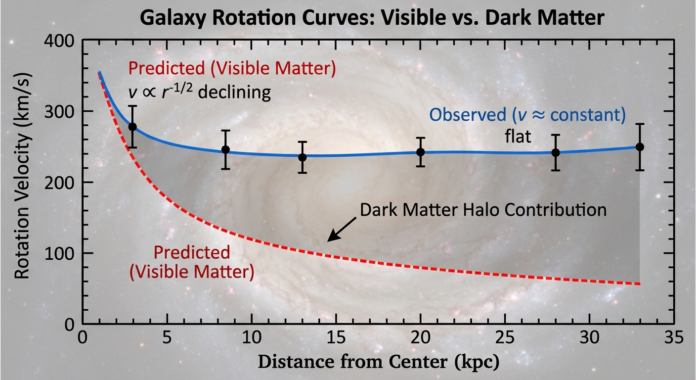
Figure 5.1: Expected (red) and Observed (blue) Galaxy Rotation Velocities
2. Gravitational Lensing
Briefly: Lensing directly measures the total mass in clusters.
Large masses bend light according to General Relativity. Lensing directly measures the total mass in clusters. Result: Total mass is ~5‑10 times the visible mass from stars and gas.
3. The Bullet Cluster
Briefly: In the collision of two galaxy clusters, X‑ray observations show hot gas, while lensing maps show that most of the mass is separated from the gas.
The most dramatic evidence! In the collision of two galaxy clusters, X‑ray observations show hot gas, while lensing maps show that most of the mass is separated from the gas. Dark matter interacts very weakly with gas.
CMB Evidence: The heights and positions of CMB acoustic peaks clearly show the difference between baryonic matter (Ωb ≈ 0.05) and dark matter (Ωc ≈ 0.27).
5.2 Dark Matter Candidates: Particle Physics Perspective
Briefly: Various theoretical models propose different particle candidates.
The microscopic nature of dark matter is one of the greatest mysteries in modern physics. Various theoretical models propose different particle candidates.
WIMPs (Weakly Interacting Massive Particles)
Briefly: They arise naturally in supersymmetry (SUSY) theories.
WIMPs were the most popular dark matter candidate from the 1980s to the 2010s. They arise naturally in supersymmetry (SUSY) theories.
Key Properties:
- Mass Range: 10 GeV - 10 TeV (weak scale)
- Interaction: Weak nuclear force scale (σ ~ 10⁻³⁶ cm²)
- Electric Charge: Neutral
- Stability: Stable on cosmological timescales
The WIMP Miracle: WIMPs produced through the thermal freeze‑out mechanism naturally give the observed dark matter density:
For weak‑scale cross‑sections (⟨σv⟩ ~ 10⁻²⁶ cm³/s), Ωχh² ≈ 0.1 is obtained — consistent with observations!
SUSY Candidates:
- Neutralino (χ⁰): Lightest supersymmetric particle (LSP), bino/wino/higgsino mixture
- Sneutrino: Neutrino superpartner (mostly excluded)
- Gravitino: Graviton superpartner (very light or very heavy)
Experimental Status (2024): Experiments like XENON1T, LUX‑ZEPLIN, PandaX‑4T have found no conclusive WIMP signal. Spin‑independent cross‑section limit: σSI < 10⁻⁴⁷ cm² (for a 100 GeV WIMP). No SUSY particles have been found at the LHC.
The WIMP Paradigm Crisis: Despite 40 years of searching, no WIMP detection has been made, prompting the community to turn to alternative candidates. However, WIMPs are not completely excluded — lighter (< 10 GeV) or heavier (> 1 TeV) masses are still possible.
Axions
Briefly: Frank Wilczek and Steven Weinberg (1978) formulated it as a particle.
The QCD axion was proposed by Roberto Peccei and Helen Quinn (1977) to solve the strong CP problem. Frank Wilczek and Steven Weinberg (1978) formulated it as a particle.
The Strong CP Problem: The QCD Lagrangian contains a term (θ‑term) that violates CP symmetry:
Neutron electric dipole moment measurements: θ < 10⁻¹⁰. Why is it so small? The Peccei‑Quinn solution makes θ a dynamical field (the axion field).
Axion Properties:
- Mass: ma ≈ 6 μeV (10¹² GeV/fa) — fa is the Peccei‑Quinn scale
- Interaction: Very weakly coupled to photons: gaγγ ~ α/(2πfa)
- Production: Misalignment mechanism (vacuum misalignment)
Cosmological Production: In the early universe, the axion field starts with a random value. Below T ~ ΛQCD, the field oscillates around the minimum (coherent oscillations):
Detection Methods:
- Haloscope (ADMX): Axion → photon conversion in a strong magnetic field, resonant cavity
- Helioscope (CAST, IAXO): Axions from the Sun
- Light‑Shining‑Through‑Wall: Laboratory experiments
Current Status: ADMX‑G2 has scanned the 2.7‑3.3 μeV range, with no signal. IAXO (2030s) will scan a wider parameter space.
Sterile Neutrinos
Briefly: They do not interact via the weak force (only gravity and neutrino mixing).
Sterile neutrinos are heavy partners of Standard Model neutrinos. They do not interact via the weak force (only gravity and neutrino mixing).
Mass Ranges:
- keV Sterile Neutrinos: ms ~ 1‑100 keV — Warm/Hot dark matter
- MeV‑GeV Sterile Neutrinos: For leptogenesis
- Heavy Neutral Leptons: ms > GeV — Seesaw mechanism
Production Mechanisms:
- Dodelson‑Widrow: Active‑sterile neutrino oscillations
- Shi‑Fuller: Resonant production (lepton asymmetry)
- Non‑thermal: Heavy particle decays
Observational Signatures:
- X‑ray Line: Sterile neutrino decay: νs → ν + γ, Eγ = ms/2
- Structure Formation: Warm dark matter suppresses small‑scale structures
The 3.5 keV Anomaly: In 2014, a 3.5 keV X‑ray line was reported in galaxy clusters (Bulbul et al., Boyarsky et al.). It is consistent with a 7 keV sterile neutrino. However, confirmation is uncertain — still debated.
Primordial Black Holes
Briefly: They are an alternative to particle dark matter.
Primordial Black Holes (PBHs) form from the collapse of density fluctuations shortly after the Big Bang. They are an alternative to particle dark matter.
Formation Mechanisms:
- Gaussian Fluctuations: Large density peaks during inflation
- Phase Transitions: QCD phase transition, electroweak phase transition
- Cosmic String Loops: Cosmic string collapse
- Bubble Collisions: In first‑order phase transitions
Mass Spectrum: PBH mass depends on formation time:
Observational Constraints:
- M < 10¹⁵ g: Hawking radiation — excluded
- 10¹⁵ - 10¹⁷ g: Femtolensing — constrained
- 10²⁰ - 10²⁴ g: Microlensing (EROS, MACHO) — excluded
- 10²⁴ - 10²⁸ g: Open window! (asteroid‑mass PBHs)
- 1‑100 M☉: LIGO/Virgo mergers — constrained but open
- > 100 M☉: CMB distortions, dynamical friction
LIGO and PBHs: LIGO's detection of black hole mergers revived the PBH dark matter hypothesis. However, detailed analyses show that all dark matter cannot be stellar‑mass PBHs (fPBH < 0.1).
SIDM: Self‑Interacting Dark Matter
Briefly: They aim to solve small‑scale structure problems.
SIDM models assume dark matter particles scatter elastically with each other. They aim to solve small‑scale structure problems.
Motivation — Small‑Scale Problems:
- Cusp‑Core Problem: N‑body simulations predict cuspy profiles in dwarf galaxies, observations show cored profiles
- Missing Satellites: ΛCDM predicts too many satellite galaxies
- Too‑Big‑To‑Fail: The largest subhalos are too dense
SIDM Cross‑Section: To be effective on galaxy scales:
This is very large by particle physics standards! (WIMP: σ/m ~ 10⁻²⁵ cm²/g)
Model Examples:
- Dark Photon: Dark U(1) gauge symmetry, light mediator boson
- Strongly Interacting Massive Particles (SIMPs): 3 → 2 annihilation
- Atomic Dark Matter: Dark atoms, dark molecules
Observational Tests:
- Galaxy Clusters: Bullet Cluster, Abell 3827 — offset measurements
- Dwarf Galaxies: Density profiles — cored vs cuspy
- Halo Shapes: SIDM produces more spherical halos
Current Status: SIDM can solve small‑scale problems, but a model consistent with all observations is not yet available. σ/m ~ 1 cm²/g is the preferred range.
Other Exotic Candidates
Briefly: Gives a concise explanation of Other Exotic Candidates.
- Fuzzy Dark Matter: Ultra‑light bosons (m ~ 10⁻²² eV), de Broglie wavelength ~ kpc
- Q‑balls: Non‑topological solitons
- Dark Photons: Kinetically mixed U(1) gauge bosons
- Asymmetric Dark Matter: Dark matter asymmetry similar to baryon asymmetry
5.3 Experimental Detection Methods
Briefly: Gives a concise explanation of Experimental Detection Methods.
Direct Detection
Briefly: Detectors: XENON1T/XENONnT, LUX, PandaX.
WIMPs passing through Earth elastically scatter off nuclei. Detectors: XENON1T/XENONnT, LUX, PandaX. Status: No conclusive signal detected. Cross‑section limits: σ < 10⁻⁴⁶ cm².
Indirect Detection
Briefly: Observations: Fermi‑LAT (gamma‑ray), AMS‑02 (cosmic ray positrons), IceCube (neutrinos).
Dark matter annihilates into Standard Model particles. Observations: Fermi‑LAT (gamma‑ray), AMS‑02 (cosmic ray positrons), IceCube (neutrinos).
Collider Searches
Briefly: Signal: "Missing energy." Status: No signal detected, supersymmetry highly constrained.
Produce dark matter particles at the LHC. Signal: "Missing energy." Status: No signal detected, supersymmetry highly constrained.
5.4 Alternative Theory: MOND
Briefly: MOND explains galaxy rotation curves without dark matter.
Mordehai Milgrom (1983): Perhaps there is no dark matter, but Newtonian dynamics is modified at low accelerations?
MOND explains galaxy rotation curves without dark matter. Critical acceleration: a₀ ≈ 1.2 × 10⁻¹⁰ m/s²
Problems with MOND
Briefly: This chapter systematically collects the tensions of ΛCDM and the observations from which they arise.
- Fails in galaxy clusters
- Cannot explain the Bullet Cluster
- Does not explain CMB or large‑scale structure formation
- Weak theoretical foundation, phenomenological
Most cosmologists do not consider MOND an alternative to dark matter.
The Greatest Puzzles in Physics and New Physics
This chapter systematically collects the tensions of ΛCDM and the observations from which they arise. The aim is to clarify which measurements motivate the search for new physics.
"Understanding the universe is one of humanity's greatest intellectual endeavors."
6.1 The Cosmological Constant Problem: The 10¹²⁰ Discrepancy
Briefly: If the cutoff is taken at the Planck scale.
According to Quantum Field Theory, "empty" space (vacuum) is filled with virtual particles. If the cutoff is taken at the Planck scale:
Observed value:
Discrepancy: 10¹²⁰ Factor! This is the worst theoretical prediction in physics! The vacuum energy must be almost exactly zero, but not exactly zero.
Possible Solutions (Speculative)
Briefly: Historical Perspective: The 1998 Shock — The Universe is Accelerating!
- Anthropic Principle: In the multiverse, life can only develop in universes where Λ is small
- Tuning Mechanism: An unknown dynamical mechanism
- Emergent Gravity: Gravity is not a fundamental force
The cosmological constant problem has been open for over 50 years, with no satisfactory solution.
Historical Perspective: The 1998 Shock — The Universe is Accelerating!
Two independent teams observed distant supernovae:
- Supernova Cosmology Project - Saul Perlmutter (Lawrence Berkeley Lab)
- High‑Z Supernova Search Team - Brian Schmidt & Adam Riess (Australian National U.)
Expectation: The universe is slowing down (due to gravity). Supernovae should be brighter than expected.
Result: Supernovae were DIMMER than expected! The universe is accelerating! (w < -1/3)
Perlmutter's comment: "My first reaction: We made a mistake. My second: Did the rival team make the same mistake? My third: Everything we know about the universe is wrong!"
Riess's memory: "I checked the data, rechecked it. But the result didn't change. The universe really was accelerating. I couldn't sleep that night."
Dark energy was discovered — 68% of the universe. Nobel Prize (2011) - Perlmutter, Schmidt, Riess.
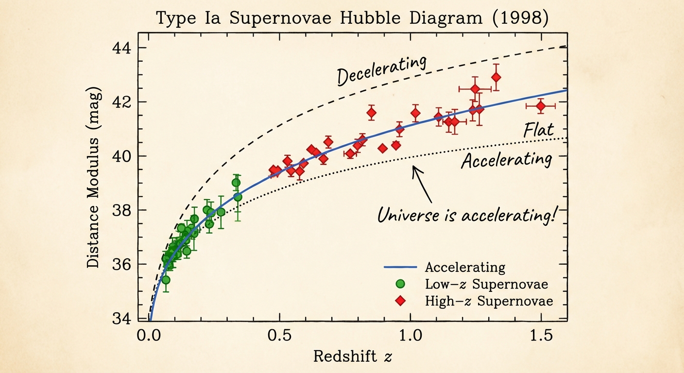
Figure 6.1: 1998 Supernova Data and an Accelerating Universe
6.1.1 Alternative Dark Energy Models
Briefly: Dynamic dark energy with a scalar field φ.
Due to the static nature of the cosmological constant and the fine‑tuning problem, dynamic dark energy models have been proposed.
Quintessence:
Dynamic dark energy with a scalar field φ:
Equation of state:
Slow‑roll: $$\frac{1}{2}\dot{\phi}^2 \ll V(\phi) \implies w \approx -1$$
Popular Quintessence Potentials:
- $$\text{V}(\phi) = V_0 e^{-\lambda\phi/M_{\text{Pl}}} \quad (\text{Tracker Behavior})$$
- $$\text{V}(\phi) = \frac{M^{4+n}}{\phi^n} \quad (\text{Freezing Models})$$
- $$\text{V}(\phi) = \Lambda^4\left[1 + \cos\left(\frac{\phi}{f}\right)\right] \quad (\text{PNGB Potential/Natural Small Mass})$$
Observational Constraints:
Planck 2018: w = -1.03 ± 0.03 (assuming constant w)
Time‑dependent: w(a) = w₀ + wa(1‑a) — CPL parametrization
K‑essence:
Scalar field with kinetic term:
Equation of state:
K‑essence affects structure formation via sound speed $$c_s^2 = \frac{P_{,X}}{P_{,X} + 2X P_{,XX}}$$.
Phantom Energy:
w < -1 equation of state — "Big Rip" scenario!
Negative kinetic energy → Phantom instability
Big Rip Time:
If w = -1.5, the universe will be torn apart in ~22 billion years!
Phantom Divide Crossing: Crossing the w = -1 boundary (phantom divide crossing) is theoretically difficult. Most scalar field models cannot achieve this transition. Observations are currently consistent with w ≈ -1, with no strong evidence for the phantom region.
Chaplygin Gas:
Generalized Chaplygin Gas (α = 1 special case):
In the early universe, it behaves like dust $$\rho \propto a^{-3}$$; at late times, like a cosmological constant (ρ → const). A unified dark matter‑energy model!
Problems:
- Sound speed $$c_s^2 = \frac{\alpha A}{\rho^{1+\alpha}}$$ — instability at high z
- Inconsistent with CMB and LSS observations
- Currently excluded (Planck + BAO)
Holographic Dark Energy:
The holographic principle: Entropy in a region is bounded by its surface area:
Dark energy density:
Where L is a characteristic length scale (Hubble horizon, particle horizon, etc.)
Choice of Hubble Horizon: L = H⁻¹
This is equivalent to a cosmological constant (w = -1).
Future Event Horizon:
This choice gives w ≠ -1 and can be tested observationally.
Model Comparison:
- ΛCDM: w = -1 (constant), simplest, Occam's Razor
- Quintessence: -1 < w < -1/3, tracker solutions
- Phantom: w < -1, Big Rip risk
- K‑essence: Kinetic dominated, sound speed effects
- Holographic: Quantum gravity connection
Current Status (2024): All observations (Planck, DES, DESI) are consistent with ΛCDM. There is no strong evidence for dynamic dark energy. However, the Hubble tension leads some researchers to consider Early Dark Energy models.
6.2 The Hubble Tension
Briefly: Crisis Status (2025): 6σ Tension!
The Hubble constant gives different results when measured by different methods:
- Early Universe (CMB - Planck): H₀ = 67.4 ± 0.5 km/s/Mpc
- Late Universe (Supernovae - SH0ES): H₀ = 73.04 ± 1.04 km/s/Mpc
Crisis Status (2025): 6σ Tension!
With the SH0ES 2024/2025 final analysis and JWST confirming Cepheid calibration, the discrepancy reached 6σ statistically. This makes a "systematic error" explanation almost impossible. The Standard Model (ΛCDM) may be cracking.
DESI 2025 and Dynamic Dark Energy
Briefly: It mapped the expansion history of the universe using Baryon Acoustic Oscillations (BAO).
DESI (Dark Energy Spectroscopic Instrument) released its first‑year (Y1) results in 2025. It mapped the expansion history of the universe using Baryon Acoustic Oscillations (BAO).
Surprising Result: The data suggest that the dark energy equation of state parameter (w) is not constant ($$w_0 > -1$$ and $$w_a \neq 0$$). If confirmed, the Cosmological Constant ($\Lambda$) idea could be falsified!
Possible Explanations
Briefly: Gives a concise explanation of Possible Explanations.
- Systematic errors (now very unlikely; JWST confirmed Cepheids)
- Early Dark Energy (EDE): Energy injection before recombination
- Dynamic Dark Energy: Time‑varying $w(z)$ (DESI hint)
- Modified Gravity (f(R), Torsion, etc.)
SH0ES Measurement Methodology
Briefly: Systematic Errors (SH0ES).
Distance Ladder:
- Parallax: Distances of nearby Cepheids measured by the Gaia satellite (d < 10 kpc)
- Cepheid Variables: Period‑Luminosity relation
$$M = -2.43 (\log P - 1) - 4.05$$
- Type Ia Supernovae: Standard candles, z ~ 0.01‑2.3
Systematic Errors (SH0ES):
- Cepheid Metallicity: Metallicity dependence of the Period‑Luminosity relation
- Crowding: Stellar crowding in galaxy centers
- Extinction: Dust extinction corrections
- Anchor Calibration: LMC distance uncertainty (±1.3%)
Planck CMB Analysis
Briefly: Planck's Advantages.
Acoustic Peaks: The positions of acoustic peaks in the CMB power spectrum determine cosmological parameters.
Planck's Advantages:
- Early universe physics (z ~ 1100)
- Model‑dependent but very precise within ΛCDM
- Systematic errors well understood
Planck's Weaknesses:
- H₀ is not measured directly; it is derived assuming ΛCDM
- If ΛCDM is wrong, H₀ is also wrong
- Lensing amplitude anomaly (A_L > 1)
Early Dark Energy (EDE)
Briefly: Effect: r_s (sound horizon) decreases → H₀ increases (consistent with Planck).
Motivation: Extra energy component before recombination changes the sound horizon.
Effect: r_s (sound horizon) decreases → H₀ increases (consistent with Planck)
Problems:
- Worsens the S₈ tension
- Conflicts with BAO measurements
- Fine‑tuning problem (why z_c ~ 10⁴?)
Modified Recombination
Briefly: Scenarios.
Scenarios:
- Extra Relativistic Species: ΔN_eff > 0 → sound horizon changes
- Primordial Magnetic Fields: Affect recombination timing
- Dark Matter‑Baryon Scattering: Acoustic peaks shift
Other Independent Measurements
Briefly: Gravitational Lensing Time Delays (H0LiCOW).
TRGB (Tip of Red Giant Branch):
- Carnegie‑Chicago Hubble Program: H₀ = 69.8 ± 1.9 km/s/Mpc
- Inconsistent with SH0ES, closer to Planck
Gravitational Lensing Time Delays (H0LiCOW):
- H₀ = 73.3 +1.7/-1.8 km/s/Mpc
- Consistent with SH0ES
BAO + BBN:
- H₀ = 67.9 ± 1.3 km/s/Mpc (DESI 2024)
- Consistent with Planck
Current Status (2024)
Briefly: JWST Observations: High‑redshift Cepheids confirm SH0ES.
DESI 2024 Results: BAO measurements support Planck (H₀ ~ 68 km/s/Mpc)
JWST Observations: High‑redshift Cepheids confirm SH0ES
Consensus: The tension is not decreasing, remaining at the 5σ level. Solutions require:
- More precise Cepheid calibration (Roman Space Telescope - 2027)
- Independent standard candles (Mira variables, masers)
- New physics models (EDE, modified gravity)
The Hubble tension is one of the most important problems in cosmology, testing the limits of the ΛCDM model.
6.3 Limitations of Inflation: Eternal Inflation and the Multiverse
Briefly: Quantum fluctuations can push the inflaton field up the potential.
Andrei Linde and Alexander Vilenkin showed that inflation never ends in some regions. Quantum fluctuations can push the inflaton field up the potential. Result: Once inflation starts, it continues forever — creating an infinite number of "pocket universes."
String Landscape and Vacuum Diversity
Briefly: Eternal inflation + string landscape → Every type of universe is realized.
String theory predicts 10⁵⁰⁰ (or more) different vacuum states. Eternal inflation + string landscape → Every type of universe is realized.
Anthropic Reasoning
Briefly: The only meaningful question is: "Why do we observe these values?" Answer: Anthropic selection — observers only exist in universes with suitable constants.
If the multiverse is real, "deriving" physical constants is meaningless. The only meaningful question is: "Why do we observe these values?" Answer: Anthropic selection — observers only exist in universes with suitable constants.
Scientific Objections:
- Untestability: We cannot access other universes
- Loss of Predictive Power: If "anything" is possible, we cannot predict anything
- Philosophy vs Physics: Is this really physics?
6.4 Alternative Cosmology: Ekpyrotic and Cyclic Models
Briefly: Gives a concise explanation of Ekpyrotic and Cyclic Models.
The Ekpyrotic Universe
Briefly: The two branes slowly approach each other; collision → Big Bang.
Justin Khoury, Paul Steinhardt (2001): The universe is born from the collision of two "branes" (higher‑dimensional objects in M‑theory). The two branes slowly approach each other; collision → Big Bang.
Advantages: Solves the flatness problem, no monopole problem. Disadvantages: Difficult to solve the horizon problem, requires M‑theory assumptions.
The Cyclic Universe
Briefly: Big Bang → Expansion → Dark energy dominance → Contraction → New Big Bang.
Paul Steinhardt and Neil Turok (2002): The universe goes through infinite cycles. Big Bang → Expansion → Dark energy dominance → Contraction → New Big Bang.
Advantages: No initial singularity problem. Disadvantages: Cycle mechanism unclear, conflicts with singularity theorems.
Bounce Cosmology
Briefly: Loop Quantum Gravity may support this scenario — quantum effects at the Planck scale prevent singularity.
Big Bounce: The universe reaches a minimum size and expands again. Loop Quantum Gravity may support this scenario — quantum effects at the Planck scale prevent singularity.
These alternative models remain speculative. They have less observational support and require more theoretical assumptions than inflation.
6.5 JWST and Early Universe Tensions (2025)
Briefly: However, its findings have created unexpected challenges for the standard ΛCDM model.
The James Webb Space Telescope (JWST) has opened a new chapter in cosmology since 2022. However, its findings have created unexpected challenges for the standard ΛCDM model.
"Impossibly Early Galaxies"
Briefly: According to the standard model, such large structures forming in such a short time is very difficult (Halo Mass Function limits).
JWST has discovered extremely bright and massive galaxies formed just 300‑400 million years after the Big Bang ($z > 10$) (e.g., JADES‑GS‑z14‑0). According to the standard model, such large structures forming in such a short time is very difficult (Halo Mass Function limits).
Mass‑Luminosity Discrepancies
Briefly: This situation requires a reevaluation of star formation efficiency and mass‑light relations.
The observed brightness of early galaxies is exceptionally high compared to their estimated stellar mass. This situation requires a reevaluation of star formation efficiency and mass‑light relations.
Possible explanations include top‑heavy IMF, brighter Pop‑III stellar populations due to low metallicity, and strong feedback mechanisms.
Toomre Stability Limits
Briefly: JWST data imply that some early disk‑like structures push the limits of standard stability criteria.
The Toomre parameter $$Q$$ is a critical criterion for disk stability. JWST data imply that some early disk‑like structures push the limits of standard stability criteria.
$$Q<1$$ regimes indicate that disks are prone to fragmentation, which could trigger rapid star formation in the early universe.
Relation to Inflation
Briefly: Possible enhancements in the small‑scale power spectrum are discussed as a mechanism that could accelerate early galaxy formation.
If early structure formation is faster than expected, this could impose indirect constraints on the amplitude or spectral index of the initial fluctuations from inflation.
Possible enhancements in the small‑scale power spectrum are discussed as a mechanism that could accelerate early galaxy formation.
Problem: The Star Formation Efficiency (SFE) in standard models is about 10‑20%. Explaining JWST data would require this ratio to be near 100% or a change in cosmology!
Possible Solutions
Briefly: Gives a concise explanation of Possible Solutions.
- Top‑Heavy IMF: The mass distribution of the first stars (Pop III) could be very different from today's (more massive stars = more light).
- Primordial Black Holes (PBH): Early black holes may have accelerated galaxy formation.
- Early Dark Energy (EDE): Changes in the expansion history of the universe could affect the timing of structure formation.
6.6 Cosmological Anomalies and Horizon‑Scale Tensions
Briefly: Gives a concise explanation of Cosmological Anomalies and Horizon‑Scale Tensions.
CMB Low‑ℓ Anomalies
Briefly: Notable anomalies include.
Planck and WMAP data show lower‑than‑expected power and specific alignments at large angular scales (ℓ < 30). Notable anomalies include:
- Quadrupole‑Octopole alignment: Unexpected orientation of the largest‑scale modes
- Hemispherical power asymmetry: Different power in the two halves of the sky
- Parity asymmetry: Imbalance between odd and even ℓ modes
The statistical significance of these anomalies is limited by cosmic variance. However, their persistence across different maps and foreground cleaning methods suggests a consistency issue worth attention.
Dipole, Quadrupole, and Octopole Problems
Briefly: This alignment may appear inconsistent with simple isotropic ΛCDM expectations.
While the dipole anisotropy is explained by observer motion, the alignment of quadrupole and octopole modes has led to the "axis of evil" debate. This alignment may appear inconsistent with simple isotropic ΛCDM expectations.
Cosmic Flow Anomalies
Briefly: Some of these results may be explained by systematic errors, but full consistency has not been achieved.
Some galaxy cluster and large‑scale structure analyses have reported larger bulk flows than predicted by standard ΛCDM. Some of these results may be explained by systematic errors, but full consistency has not been achieved.
Bulk flow magnitude constrains the large‑scale power spectrum of the velocity field and, when combined with low‑ℓ CMB anomalies, may hint at new physics scenarios.
Lensing Amplitude (AL) Tension
Planck CMB analyses have indicated that the $$A_L$$ parameter describing the lensing amplitude is greater than 1, which has been attempted to be explained by early universe physics or systematic effects.
The $$A_L > 1$$ finding implies that the lensing effect appears "excessive" in the CMB. Combined with parameter degeneracies (especially $$\Omega_m$$, $$\sigma_8$$, and $$\tau$$), this may indicate limits to model fit.
Interpretation and Possible Explanations
Briefly: Thus, anomalies are critical testbeds for both data analysis and model building.
- Systematic effects (foreground cleaning, calibration)
- Statistical fluke (cosmic variance)
- New physics in early universe dynamics (pre‑inflationary phase, isocurvature)
Alternative possibilities, such as new interactions on very small scales or a brief "pre‑inflation" period in the early universe, could also explain low‑ℓ anomalies. Thus, anomalies are critical testbeds for both data analysis and model building.
These anomalies alone do not break ΛCDM, but they are considered critical observational signals testing the model's limits.
6.7 Advanced Open Problems and New Physics
Briefly: Gives a concise explanation of Advanced Open Problems and New Physics.
Topological Defects
Briefly: Depending on the breaking topology.
Symmetry breaking in field theories can inevitably lead to topological defects. Depending on the breaking topology:
- Domain walls: Formed by discrete symmetry breaking; tightly constrained due to high energy density.
- Cosmic strings: Arise from U(1) breaking; tested by CMB and GW.
- Monopoles: Typical output of GUT breaking; require inflation for dilution.
Observational constraints (CMB anisotropies, pulsar timing, GW background) strongly limit defect densities. Nevertheless, weak signals, especially for cosmic strings, remain possible.
Early Universe Phase Transitions
Briefly: The frequency band and amplitude of these signals depend on the transition energy scale and duration.
First‑order phase transitions can generate a stochastic GW background through bubble nucleation and collisions. The frequency band and amplitude of these signals depend on the transition energy scale and duration:
If the electroweak phase transition is strongly first‑order, it could also provide a critical window for baryogenesis. Detectors such as LISA, DECIGO, and ET target these signals.
False Vacuum Decay
Briefly: In this case, the universe could transition to a lower‑energy vacuum via quantum tunneling.
The Standard Model Higgs potential may be metastable at high energies. In this case, the universe could transition to a lower‑energy vacuum via quantum tunneling:
Here $$S_E$$ is the Euclidean action, determining the vacuum lifetime. Such a transition would change physical constants and the particle spectrum, a cosmological "termination" scenario.
Modified Gravity
Briefly: Main classes include.
Instead of Λ, modifications of gravity on expansion scales have been proposed. Main classes include:
- f(R): Adding curvature functions to the Einstein‑Hilbert action.
- Horndeski/DHOST: Most general scalar‑tensor theories; second‑order equations ensure stability.
- DGP braneworld: Extra‑dimensional effects produce late‑time acceleration.
Observational tests (GW speed constraints, lensing, RSD) have significantly narrowed these models. Most scenarios require screening mechanisms (chameleon, Vainshtein).
Holographic Cosmology and Entanglement Entropy
Briefly: In cosmology, this principle translates into horizon thermodynamics and entropy calculations.
The holographic principle states that the information content of a region is proportional to its boundary area, not its volume. In cosmology, this principle translates into horizon thermodynamics and entropy calculations:
Entanglement entropy is a candidate for explaining the "micro‑degrees" of cosmological horizons. This approach offers new interpretations for early universe and dark energy problems.
Multiverse and the Measure Problem
Briefly: How to define observation probabilities (the measure problem) is uncertain.
In eternal inflation scenarios, different "pocket universes" form. How to define observation probabilities (the measure problem) is uncertain. Example measure approaches:
- Global time cutoff: A specific cosmic time slice
- Scale‑factor cutoff: Measurement according to expansion
- Causal patch: The region accessible to an observer
The choice of measure directly affects observed constants and anthropic inferences, placing it at the center of multiverse discussions.
6.8 Baryogenesis and Leptogenesis
Briefly: Electroweak baryogenesis: If the electroweak phase transition is strongly first‑order, CP violation on bubble walls can produce a net baryon asymmetry.
The matter‑antimatter asymmetry of the universe requires three Sakharov conditions:
- Baryon number violation
- C and CP violation
- Out‑of‑equilibrium processes
Electroweak baryogenesis: If the electroweak phase transition is strongly first‑order, CP violation on bubble walls can produce a net baryon asymmetry.
Leptogenesis: Decays of heavy right‑handed neutrinos produce a lepton asymmetry; this asymmetry is converted to baryon asymmetry via sphaleron processes.
This value, consistent with BBN and CMB observations, provides a strong constraint on early universe physics models.
Sphaleron Processes
Briefly: During the electroweak era, sphaleron transitions violate baryon and lepton numbers, playing a key role in transferring asymmetry from leptogenesis to the baryon sector.
During the electroweak era, sphaleron transitions violate baryon and lepton numbers, playing a key role in transferring asymmetry from leptogenesis to the baryon sector.
Sources of CP Violation
Briefly: CP violation within the SM is generally insufficient; therefore, new physics (e.g., heavy neutrino phases, extended Higgs sectors) is required.
CP violation within the SM is generally insufficient; therefore, new physics (e.g., heavy neutrino phases, extended Higgs sectors) is required.
Thermal Rates and Out‑of‑Equilibrium Condition
Briefly: This condition ensures that heavy particle decays are effective in producing asymmetry.
The out‑of‑equilibrium condition requires the decay rate to be less than the expansion rate:
This condition ensures that heavy particle decays are effective in producing asymmetry.
Future Research and Observational Projects
This chapter explains which parameters future projects will test more tightly and how they can resolve current tensions. The aim is to make visible the bridge between measurement techniques and theoretical inferences.
"Science and philosophy will combine 'how' and 'why' questions to take understanding to a higher level."
7.1 Gravitational Wave Cosmology
Briefly: Gives a concise explanation of Gravitational Wave Cosmology.
The LIGO/Virgo Revolution
Briefly: 2017: GW170817 - First neutron star merger + kilonova.
2015: First gravitational wave detection (GW150914). 2017: GW170817 - First neutron star merger + kilonova.
Cosmological Applications
Briefly: Gives a concise explanation of Cosmological Applications.
- Hubble Constant Measurement: Neutron star mergers can be used as "standard sirens"
- Primordial Gravitational Waves: Gravitational waves from inflation
- Phase Transitions: Early universe phase transitions can create a stochastic GW background
Future Detectors
Briefly: Gives a concise explanation of Future Detectors.
- LISA (Laser Interferometer Space Antenna): ESA/NASA, launch ~2035. Space‑based, million‑km arms. Will hear supermassive black hole mergers.
- Einstein Telescope (ET): Europe, underground, triangular design. 10x more sensitive than LIGO. Could see all black hole mergers up to the "dark ages" of the universe.
- Cosmic Explorer: US, 40‑km arms, L‑shaped detector. 2040s vision.
7.2 Dark Energy and Dark Matter Experiments
Briefly: Gives a concise explanation of Dark Energy and Dark Matter Experiments.
Euclid (ESA)
Briefly: Goal: Understand the nature of dark energy and dark matter.
Launch: 2023. Goal: Understand the nature of dark energy and dark matter. Methods: Weak Gravitational Lensing, Baryon Acoustic Oscillations, Galaxy Clustering. Expected: Measure the dark energy equation of state parameter w to 2% precision.
Vera Rubin Observatory (LSST)
Briefly: Will scan the sky for 10 years, imaging billions of galaxies.
Start: 2025. Will scan the sky for 10 years, imaging billions of galaxies. Goals: Type Ia supernova cosmology, weak lensing, shedding light on the Hubble tension.
Nancy Grace Roman Space Telescope (2027)
Briefly: Has the same mirror diameter as Hubble (2.4m) but a field of view 100 times wider!
NASA's next flagship mission. Has the same mirror diameter as Hubble (2.4m) but a field of view 100 times wider!
- Dark Energy: Will measure the shapes (weak lensing) and positions (BAO) of millions of galaxies.
- Exoplanets: Will discover thousands of new planets via microlensing.
- High‑Latitude Survey: Will map the expansion history of the universe with less than 1% error.
SKA (Square Kilometre Array) - The Radio Revolution
Briefly: Total collecting area of 1 km²!
The world's largest radio telescope (Australia and South Africa). Total collecting area of 1 km²!
- 21cm Cosmology: The only instrument that can map the "Dark Ages" of the universe (before the first stars).
- Gravity Tests: Will test Einstein to the limits using pulsars.
- Non‑Gaussianity: Large‑scale structure maps to distinguish inflation models.
Dark Matter Direct Detection
Briefly: Gives a concise explanation of Dark Matter Direct Detection.
- XENONnT / LZ: Liquid xenon detectors, σ < 10⁻⁴⁸ cm² sensitivity
- DARWIN: 40‑50 ton liquid xenon, neutrino floor level, 2030s
Axion Experiments
Briefly: Gives a concise explanation of Axion Experiments.
- ADMX‑G2: Scanning for axion masses 2‑40 μeV
- IAXO: Solar axion search, 2030s
7.3 CMB Polarization Measurements (Search for B‑modes)
Briefly: March 17, 2014: The BICEP2 team made a major announcement from the South Pole: "We have detected the B‑mode signal of primordial gravitational waves!
Historical Perspective: The BICEP2 Drama (2014)
March 17, 2014: The BICEP2 team made a major announcement from the South Pole: "We have detected the B‑mode signal of primordial gravitational waves! r = 0.2"
Meaning: Direct evidence for inflation theory! The media went wild. "Echoes of the Big Bang found!"
Problem: The Planck team analyzed the data. Galactic dust can produce B‑mode signals. Could BICEP2 have underestimated dust effects?
September 2014: Planck released its dust map. The BICEP2 region was dusty!
January 2015: BICEP2 and Planck joint analysis: The signal was largely from galactic dust. Only an upper limit for primordial B‑modes: r < 0.07
Lesson: The scientific process worked! The error correction mechanism kicked in. The BICEP2 team was honest and admitted the mistake. This is the strength of science.
Current status: The search for B‑modes continues. CMB‑S4, LiteBIRD, Simons Observatory...
Why Are B‑modes Important?
Briefly: Detection of B‑modes would be the "smoking gun" for inflation theory.
CMB polarization comes in two types: E‑mode (scalar fluctuations — detected) and B‑mode (tensor fluctuations — not yet detected). Detection of B‑modes would be the "smoking gun" for inflation theory.
BICEP/Keck Array
Briefly: Planck + BICEP2/Keck (2018): r < 0.036.
BICEP2 (2014): "B‑mode detected!" — False alarm (galactic dust). Planck + BICEP2/Keck (2018): r < 0.036
Future CMB Experiments
Briefly: Space‑based CMB polarization satellite.
LiteBIRD (JAXA/ESA - 2028+):
Space‑based CMB polarization satellite. Single goal: Find B‑modes or exclude r < 0.001. The biggest hope for the "smoking gun" of inflation.
CMB‑S4 (Stage 4):
A ground‑based network to be deployed in Chile and at the South Pole. 500,000 superconducting detectors. Will also make precise measurements for neutrino masses and dark matter.
Simons Observatory (2024/2025):
The precursor to CMB‑S4. Currently taking data! Expected to reach r ~ 0.003 sensitivity.
Significance of r Detection:
- r > 0.01: Large‑field inflation — Trans‑Planckian physics!
- r ~ 0.001: Plateau‑type models (Starobinsky, Higgs)
- r < 0.001: Small‑field inflation — detection difficult
7.4 Major Observational Projects Through the 2030s
Briefly: For example, Euclid's weak lensing data combined with Roman's supernova measurements will provide strong constraints on $$w(z)$$ parametrizations.
- Euclid: Geometric mapping of dark energy and structure formation
- Roman: Wide‑field supernova and weak lensing programs
- SKA: 21 cm cosmology and mapping the dark ages
- JWST continuation programs: Early galaxy populations and reionization
- LISA: Cosmic gravitational‑wave background
These projects aim to break parameter degeneracies by combining different observational windows. For example, Euclid's weak lensing data combined with Roman's supernova measurements will provide strong constraints on $$w(z)$$ parametrizations. SKA opens a direct window to structure formation at high redshifts through the 21 cm signal.
7.5 New Measurement Techniques and Standard Sirens
Briefly: 21 cm Cosmology: The neutral hydrogen signal from the dark ages allows direct measurement of the growth history of the early universe.
Standard Sirens: Gravitational waves directly measure distance:
21 cm Cosmology: The neutral hydrogen signal from the dark ages allows direct measurement of the growth history of the early universe.
CMB Stage‑IV: Provides major sensitivity improvements in neutrino mass, B‑modes, and lensing measurements.
Ultra‑Deep BAO: Large‑volume BAO surveys will constrain geometry with high precision.
In the standard siren approach, if an electromagnetic counterpart (kilonova/host galaxy) is found, it can be matched with redshift, reducing dependence on the classical distance ladder and providing an independent measurement of H₀.
7.6 Artificial Intelligence in Parameter Inference
Briefly: Emulators: Fast predictors that mimic CAMB/CLASS outputs.
Bayesian Inference + ML: Emulators and surrogate models are used to accelerate MCMC chains.
Emulators: Fast predictors that mimic CAMB/CLASS outputs.
Deep Generative Models: Used to sample likelihood surfaces and scan parameter spaces.
Likelihood‑free Inference: Simulation‑based inference (SBI) is useful when an explicit likelihood cannot be written. Normalizing flow and diffusion‑based models directly produce posterior distributions.
Risks: ML emulators may produce errors outside their training range, and "black box" models may hide systematics. Therefore, validation sets, physical priors, and coverage tests are essential.
These methods speed up parameter estimation on large datasets while redefining the risks of systematic errors and model dependence.
Quantum Cosmology and the Beginning of the Universe
This chapter discusses the singularity and time problems of classical cosmology within a quantum framework. The aim is to show which observational signatures of Planck‑scale effects can be tested and to physically understand the "beginning" question.
"How did everything begin, or was there no beginning at all?"
8.1 The Wheeler‑DeWitt Equation: Wave Function of the Universe
Briefly: Quantum cosmology attempts to give a quantum mechanical description of the universe.
Classical General Relativity fails at the Big Bang singularity (ρ → ∞, a → 0). Quantum cosmology attempts to give a quantum mechanical description of the universe.
Hamiltonian Formulation
Briefly: Here N is the lapse function, N^i is the shift vector, and h_ij is the 3‑metric.
ADM (Arnowitt‑Deser‑Misner) Formalism: Splits spacetime into 3+1 dimensions:
Here N is the lapse function, N^i is the shift vector, and h_ij is the 3‑metric.
The Wheeler‑DeWitt Equation
Briefly: Minisuperspace Approach: Only the scale factor a(t) and homogeneous scalar field φ.
For the wave function of the universe $$\Psi[h_{ij}, \phi]$$:
Minisuperspace Approach: Only the scale factor a(t) and homogeneous scalar field φ:
Problems:
- Problem of Time: No time in the equation! ∂Ψ/∂t = 0
- Boundary Conditions: What happens at a = 0?
- Interpretation: What does |Ψ|² represent?
The Hartle‑Hawking "No‑Boundary" Proposal
Briefly: In 1983, Stephen Hawking and James Hartle collaborated at Cambridge.
Historical Perspective: Hawking & Hartle — "The Universe Has No Boundary"
In 1983, Stephen Hawking and James Hartle collaborated at Cambridge. The question: How did the universe begin? How to overcome the Big Bang singularity?
Radical idea: "The universe has no boundary!" (No‑Boundary Proposal)
In imaginary time (t → -iτ), the universe begins like the "South Pole." No singularity, just a smooth geometry. Time emerges from space!
Hawking's metaphor: "It's like asking what is north of the North Pole. The question is meaningless. So is the question of what came before the beginning of the universe."
Philosophy vs Physics: Is this testable? Hawking: "Yes! It could leave traces in the CMB."
Debate: Competes with Vilenkin's tunneling proposal. Which is correct? We don't know yet.
Legacy: Hawking died in 2018. His last paper (2018): "Smooth exit from eternal inflation?" Attempted to constrain the multiverse. The question remains open...
Idea: The universe has no boundary; Euclidean path integral:
In imaginary time (t → -iτ), the universe begins like the "South Pole" — no singularity!
Vilenkin Tunneling Proposal
Briefly: Here S_E is the Euclidean action.
Alternative: The universe tunnels into existence from "nothing":
Here S_E is the Euclidean action. The universe tunnels from a classically forbidden region.
Philosophy: The Wheeler‑DeWitt equation attempts to explain the "creation" of the universe with quantum mechanics. However, the problem of time and interpretational difficulties remain.
8.2 Loop Quantum Cosmology (LQC): Quantization of Spacetime
Briefly: Fundamental building blocks: spin networks.
Loop Quantum Gravity (LQG): Spacetime itself is quantized. Fundamental building blocks: spin networks.
Basic Ideas of LQC
Briefly: Holonomy‑Flux Variables: Instead of classical (a, ȧ).
Holonomy‑Flux Variables: Instead of classical (a, ȧ):
- Holonomy: h = exp(c/2) ~ connection
- Flux: p ~ a² (volume)
Quantization:
Modified Friedmann Equation
Briefly: Where the critical density is.
In LQC, the Friedmann equation is modified:
Where the critical density is:
Result: As ρ → ρ_crit, H → 0! The Big Bang singularity is resolved.
Quantum Bounce
Briefly: Minimum Scale Factor.
Scenario:
- The universe contracts (a → a_min)
- As ρ → ρ_crit, quantum effects dominate
- Gravitational attraction → repulsive gravity!
- The universe "bounces" and begins to expand
Minimum Scale Factor:
Typically: a_min ~ 10⁻³⁵ m (around the Planck length)
The Pre‑Big Bang Universe
Briefly: Information Transfer: Is information preserved during the bounce?
Cyclic Universe: LQC allows for a "previous universe" before the bounce:
- The previous universe contracts
- Quantum transition at the bounce point
- Our universe expands
Information Transfer: Is information preserved during the bounce? Debatable!
Advantages of LQC:
- Singularity resolved — mathematically robust
- Makes predictions at the Planck scale
- Can explain pre‑inflation dynamics
Problems:
- Full LQG theory is not yet complete
- Observational tests are very difficult
- Anisotropies and inhomogeneities not fully understood
8.3 Observational Effects of Quantum Fluctuations
Briefly: Gives a concise explanation of Observational Effects of Quantum Fluctuations.
Quantum Imprints in the CMB
Briefly: Here k_Pl ~ 10²³ Mpc⁻¹ (Planck momentum scale).
Primordial Power Spectrum Corrections: LQC bounce predicts corrections to the power spectrum:
Here k_Pl ~ 10²³ Mpc⁻¹ (Planck momentum scale)
Observational Constraints:
- Planck 2018: Primordial power spectrum nearly perfect power‑law
- Upper limit on quantum corrections: |α| < 10⁻²
- No direct trace of LQC bounce in the CMB (yet)
Primordial Gravitational Waves
Briefly: Tensor Mode: The bounce affects the primordial gravitational wave spectrum.
Tensor Mode: The bounce affects the primordial gravitational wave spectrum:
- Corrections at high frequencies (f > 10⁻¹⁶ Hz)
- Bounce signature: "break" in the spectrum
- Future: Can be tested with LISA, Einstein Telescope
The Trans‑Planckian Problem
Briefly: Quantum gravity effects must be present!
Problem: The CMB modes we observe today, at the beginning of inflation, were smaller than the Planck scale (λ < ℓ_Pl). Quantum gravity effects must be present!
LQC Solution: The universe before the bounce "pre‑stretches" the modes → alleviates the Trans‑Planckian problem.
Future Observations
Briefly: Primordial Black Holes.
CMB Polarization (B‑modes):
- CMB‑S4, LiteBIRD: r < 0.001 sensitivity
- Quantum corrections could affect r
21‑cm Cosmology:
- Observations of the dark ages (z ~ 30‑1100)
- Bounce signature: anomalies in the power spectrum
Primordial Black Holes:
- The bounce could affect PBH formation
- LIGO/Virgo/KAGRA: Mass spectrum tests
Current Status (2024): Quantum cosmology has advanced theoretically, but there is no observational evidence yet. In the next 10 years, CMB polarization, gravitational waves, and 21‑cm observations could test Planck‑scale physics. LQC bounce is the most promising singularity resolution scenario.
8.4 Stochastic Inflation and Decoherence
Briefly: Here $$\xi(t)$$ is a white noise term, giving a Langevin‑like stochastic dynamic.
During inflation, long‑wavelength modes become classical and form a stochastic background.
Here $$\xi(t)$$ is a white noise term, giving a Langevin‑like stochastic dynamic. This approach explains how quantum fluctuations during inflation seed classical structures.
This Langevin equation is equivalent to a Fokker‑Planck form that gives the time evolution of the probability distribution:
IR Cutoff Problem
Briefly: Thus, a physical cutoff scale or observational window function is needed.
The contribution of very long wavelengths can lead to IR divergences in theory. Thus, a physical cutoff scale or observational window function is needed.
The IR cutoff is defined in practice by the observer horizon or a finite‑volume simulation box. The chosen cutoff affects the power spectrum of long‑wavelength modes.
Decoherence and Classicalization
Briefly: This explains the emergence of the "classical universe" on cosmological scales.
Interaction with the environment (gravitons, other fields) erases the phase information of quantum modes, producing classical statistical distributions. This explains the emergence of the "classical universe" on cosmological scales.
Decoherence suppresses quantum interference terms for super‑horizon modes. Thus, the statistical properties of the CMB become consistent with a classical Gaussian field approach.
8.5 The Information Problem and the Arrow of Time
Briefly: How is information conservation interpreted within cosmic singularities and quantum gravity?
A fundamental question in quantum cosmology: Is the wave function of the universe unitary? How is information conservation interpreted within cosmic singularities and quantum gravity?
- Entropy: The low‑entropy beginning of the universe determines the arrow of time.
- Unitarity: Quantum cosmology debates whether information loss occurs.
- Absence of Time: The lack of a time parameter in the Wheeler‑DeWitt equation leads to the idea of "emergent time."
The increase in entropy determines the cosmic arrow and is directly related to black hole entropy and cosmological horizon thermodynamics. Therefore, the information problem in cosmology affects not only initial conditions but also the long‑term fate of the universe.
Alternative approaches argue that time emerges from entanglement structures. This view treats time as a derived quantity, not fundamental.
This problem area lies at the intersection of cosmology and quantum information theory and is one of the deepest debates in modern cosmology.
CONCLUSION: The Golden Age of Cosmology
Modern cosmology is experiencing an extraordinary period observationally and theoretically. In the last 30 years, we have discovered that the universe is accelerating, mapped the CMB with precision, detected gravitational waves, and confirmed the existence of dark matter through multiple methods.
But deep mysteries remain: What is dark matter? What is dark energy? Is the Hubble tension real? Is inflation correct? Is the multiverse real?
In the next 10‑20 years, next‑generation telescopes and experiments (JWST, Euclid, Vera Rubin, CMB‑S4, LISA, xenon detectors) may answer many of these questions.
Cosmology continues to push the limits of human understanding. From the beginning to the end of the universe, from the smallest quantum fluctuations to the largest structures, we are trying to understand the nature of reality.
Ad astra per aspera
Through hardships to the stars
Fundamental Constants and Resources
This section collects the technical infrastructure needed for derivations and data analysis in one place. The aim is to make the mathematical and numerical basis of the physical claims in the main text quickly accessible.
APPENDIX A: Fundamental Physical Constants
Briefly: Gives a concise explanation of Fundamental Physical Constants.
- Speed of light: c = 299,792,458 m/s
- Planck's constant: ℏ = 1.055 × 10⁻³⁴ J·s
- Newton's constant: G = 6.674 × 10⁻¹¹ m³/(kg·s²)
- Boltzmann constant: kB = 1.381 × 10⁻²³ J/K
Planck Units
Briefly: Gives a concise explanation of Planck Units.
- Planck length: lP ≈ 1.6 × 10⁻³⁵ m
- Planck time: tP ≈ 5.4 × 10⁻⁴⁴ s
- Planck mass: MP ≈ 2.2 × 10⁻⁸ kg ≈ 1.22 × 10¹⁹ GeV/c²
Cosmological Parameters (Planck 2018)
Briefly: Gives a concise explanation of Cosmological Parameters.
- Hubble constant: H₀ = 67.4 ± 0.5 km/s/Mpc
- Age of the universe: t₀ = 13.787 ± 0.020 billion years
- CMB temperature: TCMB = 2.7255 ± 0.0006 K
APPENDIX B: Further Reading and Bibliography
Briefly: Gives a concise explanation of Further Reading and Bibliography.
Classic Papers (Historical Significance)
Briefly: Gives a concise explanation of Classic Papers.
- Friedmann, A. (1922): "Über die Krümmung des Raumes" - First expanding universe solution
- Lemaître, G. (1927): "Un Univers homogène de masse constante" - Hubble law derivation
- Einstein, A. (1917): "Kosmologische Betrachtungen zur allgemeinen Relativitätstheorie" - Cosmological constant
- Hubble, E. (1929): "A Relation Between Distance and Radial Velocity" - Galaxy recession velocities
- Penzias, A. & Wilson, R. (1965): "A Measurement of Excess Antenna Temperature at 4080 Mc/s" - CMB discovery
- Guth, A. (1981): "Inflationary Universe: A Possible Solution to the Horizon and Flatness Problems"
- Peccei, R. & Quinn, H. (1977): "CP Conservation in the Presence of Pseudoparticles" - Axion theory
Modern Foundational Works
Briefly: Gives a concise explanation of Modern Foundational Works.
- Perlmutter, S. et al. (1999): "Measurements of Ω and Λ from 42 High‑Redshift Supernovae" - Accelerating universe
- Riess, A. et al. (1998): "Observational Evidence from Supernovae for an Accelerating Universe" - Nobel 2011
- Planck Collaboration (2018): "Planck 2018 results. VI. Cosmological parameters" - Most precise CMB measurements
- WMAP Team (2013): "Nine‑Year Wilkinson Microwave Anisotropy Probe (WMAP) Observations"
- Rubin, V. & Ford, W. (1970): "Rotation of the Andromeda Nebula" - Dark matter evidence
- Clowe, D. et al. (2006): "A Direct Empirical Proof of the Existence of Dark Matter" - Bullet Cluster
Recent Developments (2020‑2025)
Briefly: Gives a concise explanation of Recent Developments.
- DESI Collaboration (2024): "DESI 2024 VI: Cosmological Constraints from the Measurements of Baryon Acoustic Oscillations"
- NANOGrav Collaboration (2023): "The NANOGrav 15 yr Data Set: Evidence for a Gravitational‑wave Background"
- JWST Collaboration (2023‑2024): "JWST Advanced Deep Extragalactic Survey" - High‑redshift galaxies
- Euclid Collaboration (2024): "Euclid preparation: First Release" - First weak lensing results
- Riess, A. et al. (2022): "A Comprehensive Measurement of the Local Value of the Hubble Constant" - H₀ = 73.04 ± 1.04
- LUX‑ZEPLIN Collaboration (2023): "First Dark Matter Search Results from the LUX‑ZEPLIN Experiment"
- ADMX Collaboration (2024): "Extended Search for the Invisible Axion with ADMX"
Theoretical Reviews and Books
Briefly: Gives a concise explanation of Theoretical Reviews and Books.
- Cosmology - Steven Weinberg (2008) - Comprehensive theoretical resource
- Modern Cosmology - Scott Dodelson & Fabian Schmidt (2020) - Current standard
- Physical Foundations of Cosmology - Viatcheslav Mukhanov (2005)
- The Early Universe - Edward Kolb & Michael Turner (1990) - Classic reference
- Introduction to Cosmology - Barbara Ryden (2016) - Introductory level
- Particle Dark Matter - Gianfranco Bertone (Ed.) (2010)
- Inflation and String Theory - Daniel Baumann & Liam McAllister (2015)
Modified Gravity and Alternative Theories
Briefly: Gives a concise explanation of Modified Gravity and Alternative Theories.
- Starobinsky, A. (1980): "A New Type of Isotropic Cosmological Models" - f(R) inflation
- Brans, C. & Dicke, R. (1961): "Mach's Principle and a Relativistic Theory of Gravitation"
- Horndeski, G. (1974): "Second‑order scalar‑tensor field equations in a four‑dimensional space"
- Milgrom, M. (1983): "A Modification of the Newtonian Dynamics" - MOND
- Nicolis, A. et al. (2009): "The Galileon as a local modification of gravity" - Galileon theory
- Clifton, T. et al. (2012): "Modified Gravity and Cosmology" - Comprehensive review
Dark Matter Candidates
Briefly: Gives a concise explanation of Dark Matter Candidates.
- Jungman, G. et al. (1996): "Supersymmetric Dark Matter" - WIMP review
- Wilczek, F. (1978): "Problem of Strong P and T Invariance" - Axion naming
- Dodelson, S. & Widrow, L. (1994): "Sterile Neutrinos as Dark Matter" - Sterile neutrino production
- Carr, B. & Kühnel, F. (2020): "Primordial Black Holes as Dark Matter" - PBH review
- Tulin, S. & Yu, H. (2018): "Dark Matter Self‑interactions and Small Scale Structure" - SIDM
- Hui, L. et al. (2017): "Ultralight Scalars as Cosmological Dark Matter" - Fuzzy DM
Dark Energy and the Cosmological Constant
Briefly: Gives a concise explanation of Dark Energy and the Cosmological Constant.
- Weinberg, S. (1989): "The Cosmological Constant Problem" - Classic review
- Caldwell, R. et al. (1998): "Cosmological Imprint of an Energy Component with General Equation of State" - Quintessence
- Caldwell, R. (2002): "A Phantom Menace? Cosmological Consequences of a Dark Energy Component" - Phantom energy
- Li, M. (2004): "A Model of Holographic Dark Energy" - Holographic dark energy
Inflation Theory
Briefly: Gives a concise explanation of Inflation Theory.
- Linde, A. (1982): "A New Inflationary Universe Scenario" - Chaotic inflation
- Mukhanov, V. & Chibisov, G. (1981): "Quantum Fluctuations and a Nonsingular Universe" - Quantum fluctuations
- Lyth, D. & Riotto, A. (1999): "Particle Physics Models of Inflation" - Review article
- Baumann, D. (2009): "TASI Lectures on Inflation" - Pedagogical resource
- Planck Collaboration (2020): "Planck 2018 results. X. Constraints on inflation" - Observational constraints
Gravitational Waves and Cosmology
Briefly: Gives a concise explanation of Gravitational Waves and Cosmology.
- LIGO/Virgo Collaboration (2016): "Observation of Gravitational Waves from a Binary Black Hole Merger" - GW150914
- LIGO/Virgo Collaboration (2017): "GW170817: Observation of Gravitational Waves from a Binary Neutron Star Inspiral"
- Abbott, B. et al. (2017): "Gravitational Waves and Gamma‑Rays from a Binary Neutron Star Merger" - Multi‑messenger astronomy
- Caprini, C. & Figueroa, D. (2018): "Cosmological Backgrounds of Gravitational Waves" - Review
Online Resources and Databases
Briefly: Gives a concise explanation of Online Resources and Databases.
- arXiv.org (astro‑ph.CO): Cosmology preprints
- NASA/IPAC Extragalactic Database (NED): Galaxy database
- Particle Data Group: Cosmological parameter summary
- Planck Legacy Archive: CMB maps and data
- CAMB/CLASS: Boltzmann code libraries
- CosmoMC: MCMC parameter estimation
Major Research Groups and Projects
Briefly: Gives a concise explanation of Major Research Groups and Projects.
- Planck Collaboration (ESA)
- LIGO/Virgo/KAGRA Collaboration
- Dark Energy Survey (DES)
- Sloan Digital Sky Survey (SDSS/BOSS/eBOSS/DESI)
- Euclid Mission (ESA)
- Vera Rubin Observatory (LSST)
- James Webb Space Telescope (JWST)
- Simons Observatory & CMB‑S4
APPENDIX C: Essential Equation Derivations (For Researchers)
Briefly: Gives a concise explanation of Essential Equation Derivations.
C.1: Derivation of the Friedmann Equations
Briefly: Christoffel Symbols (important ones).
Einstein Field Equations:
FLRW Metric:
Christoffel Symbols (important ones):
- $$\Gamma^{0}_{ij} = \frac{\dot{a}}{c^2} a g_{ij}$$
- $$\Gamma^{i}_{j0} = \frac{\dot{a}}{a} \delta^{i}_{j}$$
Ricci Tensor Components:
Ricci Scalar:
Energy‑Momentum Tensor (perfect fluid):
00 Component of the Einstein Equation:
First Friedmann Equation:
ij Component of the Einstein Equation:
Second Friedmann Equation:
C.2: Cosmological Distance Measures
Briefly: Where $$H(z) = H_0 \sqrt{\Omega_m(1+z)^3 + \Omega_r(1+z)^4 + \Omega_k(1+z)^2 + \Omega_\Lambda}$$.
Comoving Distance:
Where $$H(z) = H_0 \sqrt{\Omega_m(1+z)^3 + \Omega_r(1+z)^4 + \Omega_k(1+z)^2 + \Omega_\Lambda}$$
Angular Diameter Distance:
Luminosity Distance:
Distance Modulus (Supernova Cosmology):
Comoving Distance in Curved Space:
- $$d_C = \int_{0}^{z} \frac{c \, dz'}{H(z')} \quad \text{If } k = 0 \text{ (Flat Space)}$$
- $$d_C = \frac{c}{\sqrt{\Omega_k} H_0} \sin\left[\sqrt{\Omega_k} H_0 \int_{0}^{z} \frac{dz'}{H(z')}\right] \quad \text{If } k > 0 \text{ (Closed/Spherical Space)}$$
- $$d_C = \frac{c}{\sqrt{|\Omega_k|} H_0} \sinh\left[\sqrt{|\Omega_k|} H_0 \int_{0}^{z} \frac{dz'}{H(z')}\right] \quad \text{If } k < 0 \text{ (Open/Hyperbolic Space)}$$
C.3: Fundamentals of Perturbation Theory
Briefly: Linear Perturbation Equation (Matter Dominated).
Metric Perturbations (Newtonian Gauge):
Density Contrast:
Linear Perturbation Equation (Matter Dominated):
Growth Factor:
In the matter‑dominated era: $$D(a) \propto a$$ (Einstein‑de Sitter)
Transfer Function:
Power Spectrum:
Eisenstein‑Hu Transfer Function (approximate):
Where $$q = \frac{k}{\Omega_m h^2 \, \text{Mpc}^{-1}}$$
C.4: CMB Physics Formulas
Briefly: Acoustic Peak Positions.
Sachs‑Wolfe Effect (large scales):
Acoustic Peak Positions:
Where $$\theta_s = \frac{r_s}{d_A(z_*)}$$ is the sound horizon angle
Sound Horizon:
Sound Speed (Baryon‑Photon Plasma):
Where $$R_b = \frac{3\rho_b}{4\rho_\gamma} = \frac{0.75 \Omega_b}{\Omega_\gamma a}$$
Silk Damping Scale:
Polarization (E‑mode, B‑mode):
- E‑mode: From scalar perturbations (density fluctuations)
- B‑mode: From tensor perturbations (primordial gravitational waves)
Tensor‑Scalar Ratio:
Where ε = (MPl²/16π)(V'/V)² is the slow‑roll parameter
APPENDIX D: Numerical Methods and Computational Tools (For Researchers)
Briefly: Gives a concise explanation of Numerical Methods and Computational Tools.
D.1: Boltzmann Solvers
Briefly: Example CAMB Usage (Python).
CAMB (Code for Anisotropies in the Microwave Background):
- Language: Fortran 90 (Python wrapper available)
- Use: CMB power spectrum, matter power spectrum calculation
- Input: Cosmological parameters (H₀, Ωb, Ωc, ns, τ, As)
- Output: CℓTT, CℓEE, CℓTE, P(k)
- Installation: pip install camb
Example CAMB Usage (Python):
pars = camb.CAMBparams()
pars.set_cosmology(H0=67.5, ombh2=0.022, omch2=0.122)
pars.InitPower.set_params(ns=0.965, As=2e-9)
results = camb.get_results(pars)
powers = results.get_cmb_power_spectra(pars)
CLASS (Cosmic Linear Anisotropy Solving System):
- Language: C (Python wrapper: classy)
- Advantages: More modular, extensible
- Features: Neutrino masses, modified gravity support
- Installation: pip install classy
D.2: N‑body Simulations
Briefly: Tree Algorithm (Barnes‑Hut).
Particle‑Mesh (PM) Method:
- Assign particles to grid (CIC, NGP, TSC)
- Solve Poisson equation (FFT)
- Force interpolation
- Particle motion (Leap‑frog integrator)
Tree Algorithm (Barnes‑Hut):
- Octree data structure
- Multipole expansion
- Opening criterion: θ = s/d < θmax
Popular N‑body Codes:
- GADGET‑2/4: TreePM hybrid, SPH hydrodynamics
- RAMSES: AMR (Adaptive Mesh Refinement)
- Enzo: AMR + hydrodynamics + chemistry
- PKDGRAV: Large‑scale structure simulations
Initial Conditions (Zeldovich Approximation):
Where Ψ(q) = -∇Φ(q)/(4πGρ̄a²) is the displacement field
D.3: Monte Carlo Methods
Briefly: Monte Carlo estimate of an integral.
Basic Monte Carlo Integration:
Monte Carlo estimate of an integral:
Where xi ~ U(a,b) are sampled from a uniform distribution.
Error Estimate:
The Monte Carlo error scales as N⁻¹/² — independent of dimension!
Cosmological Application — Volume Integral:
Monte Carlo is very effective for high‑dimensional integrals.
Importance Sampling:
Using a weighted distribution for better sampling:
Where $x_i \sim g(x)$ are sampled. Optimal: $g(x) \propto |f(x)|$
Error Propagation:
Propagation of parameter uncertainties to results:
- 1. Sample parameters from their distributions: $\theta_i \sim p(\theta)$
- 2. Compute result for each sample: $y_i = f(\theta_i)$
- 3. Analyze result distribution: mean(y), std(y), percentiles
Example: H₀ Uncertainty Propagated to Distance:
# H₀ uncertainty: 67.4 ± 0.5 km/s/Mpc
H0_samples = np.random.normal(67.4, 0.5, 10000)
# Luminosity distance at z=1
z = 1.0
d_L = (c/H0_samples) * (1+z) * integral(z)
# Result distribution
print(f"d_L = {np.mean(d_L):.1f} ± {np.std(d_L):.1f} Mpc")
Bootstrap Method:
Uncertainty estimation by resampling the dataset:
- 1. Draw N points from N data points (with replacement)
- 2. Compute the statistic on the bootstrap sample
- 3. Repeat B times (typically B = 1000‑10000)
- 4. Find confidence intervals from the bootstrap distribution
Cosmological Application — Supernova Fit:
results = []
for i in range(B):
# Resample data
idx = np.random.choice(len(data), len(data))
boot_data = data[idx]
# Fit cosmology
Om, Ol = fit_cosmology(boot_data)
results.append([Om, Ol])
return np.array(results)
Rejection Sampling:
Sampling from complex distributions:
- 1. Sample x ~ g(x) (proposal distribution)
- 2. Draw u ~ U(0, M g(x))
- 3. If u < f(x), accept x; otherwise reject
Where M g(x) ≥ f(x) everywhere.
Variance Reduction Techniques:
- Antithetic Variables: Use x and 1‑x together
- Control Variates: Use a known integral as a reference
- Stratified Sampling: Divide the region into strata
- Quasi‑Monte Carlo: Low‑discrepancy sequences (Sobol, Halton)
Practical Recommendations:
- Start with N > 10,000 samples
- Perform convergence tests (increase sample size)
- Reduce variance with importance sampling
- In high dimensions (d > 5), Monte Carlo is better than deterministic methods
- Ideal for parallel computing (embarrassingly parallel)
D.4: MCMC Parameter Estimation
Briefly: Likelihood Function (for CMB).
Metropolis‑Hastings Algorithm:
- 1. Choose initial parameters θ₀
- 2. Propose new parameters: $$\theta' \sim q(\theta'|\theta)$$
- 3. Compute acceptance ratio: $$\alpha = \min\left[1, \frac{L(\theta')\pi(\theta')}{L(\theta)\pi(\theta)}\right]$$
- 4. Draw $$u \sim U(0,1)$$; if $$u < \alpha$$, set $$\theta_{i+1}=\theta'$$; otherwise $$\theta_{i+1}=\theta$$
- 5. Repeat
Likelihood Function (for CMB):
CosmoMC:
- CAMB‑based MCMC code
- Planck, WMAP, BAO, SNe datasets
- Gelman‑Rubin convergence test
- GetDist analysis tools
emcee (Python MCMC):
- Affine‑invariant ensemble sampler
- Parallel computation support
- Easy to use
D.5: Integration Techniques
Briefly: Python Example (Luminosity Distance).
Cosmological Distance Integration:
Numerical Methods:
- Simpson's Rule: O(h⁴) error
- Romberg Integration: Richardson extrapolation
- Gauss‑Legendre Quadrature: High precision
- Adaptive Quadrature: scipy.integrate.quad
Python Example (Luminosity Distance):
import numpy as np
def E(z, Om, Ol):
return np.sqrt(Om*(1+z)**3 + Ol)
def d_L(z, H0, Om, Ol):
c = 299792.458 # km/s
integral, _ = quad(lambda zp: 1/E(zp, Om, Ol), 0, z)
return (c/H0) * (1+z) * integral
Boltzmann Equation Integration:
- Runge‑Kutta 4th order (RK4)
- Bulirsch‑Stoer method
- Stiff ODE solvers (LSODA)
D.6: Data Analysis Tools
Briefly: Corner Plots (Parameter Constraints).
HEALPix (CMB Maps):
- Spherical harmonic analysis
- Equal‑area pixelation
- Fast spherical harmonic transform
Astropy (Python):
- Cosmology calculations (astropy.cosmology)
- Unit conversions
- FITS file handling
Corner Plots (Parameter Constraints):
- corner.py (Python)
- GetDist (with CosmoMC)
- 1D and 2D posterior distributions
Practical Recommendations:
- Start with CAMB/CLASS — standard tools
- For MCMC, discard the burn‑in period (first 20‑30%)
- Perform convergence tests (Gelman‑Rubin R < 1.1)
- Choose softening length carefully for N‑body simulations
- Use adaptive methods for numerical integration
D.7: Bayesian Statistics and Model Comparison
Briefly: Cosmological Application.
Bayes' Theorem:
Where:
- P(θ|D): Posterior (parameter distribution given data)
- P(D|θ): Likelihood (probability of data given parameters)
- P(θ): Prior (parameter knowledge before data)
- P(D): Evidence (model evidence, normalization)
Cosmological Application:
Prior Selection:
- Uniform (Flat): π(θ) = const — Uninformative prior
- Jeffreys: π(θ) ∝ √det[I(θ)] — Reparametrization invariant
- Informative: From previous observations (e.g., BBN → $\Omega_b h^2$)
- Physical: Physical constraints (e.g., $0 < \Omega_m$ < 1)
Evidence Calculation:
Evidence measures how well a model explains the data over all parameter space.
Bayes Factor (Model Comparison):
Jeffreys Scale:
- ln B < 1: Weak evidence
- 1 < ln B < 2.5: Moderate evidence
- 2.5 < ln B < 5: Strong evidence
- ln B > 5: Very strong evidence
Example: ΛCDM vs wCDM:
Planck 2018 data: ln B(ΛCDM/wCDM) ≈ 2.3 → ΛCDM is preferred (Occam's Razor)
Information Criteria (Approximate Methods):
AIC (Akaike Information Criterion):
Where k is the number of parameters. Lower AIC is better.
BIC (Bayesian Information Criterion):
Where N is the number of data points. BIC penalizes complex models more heavily.
Model Comparison Example:
# wCDM: k=7 (+ w)
ΔBIC = BIC_wCDM - BIC_ΛCDM
# If ΔBIC > 2, ΛCDM is preferred
Bayesian Model Averaging:
Weighted average of multiple models:
Model posterior probability:
Tension Metrics:
Inconsistency between two datasets:
T > 3σ: Significant tension (e.g., Hubble tension: T ≈ 5σ)
Practical Recommendations:
- Clearly state and justify prior choices
- Perform prior sensitivity analysis
- Use nested sampling for evidence calculation (MultiNest, PolyChord)
- Use both Bayes factor and AIC/BIC for model comparison
- Perform posterior predictive checks (model validation)
D.8: Observational Techniques
Briefly: Gives a concise explanation of Observational Techniques.
Photometric Redshift (Photo‑z)
Briefly: Template Fitting Method.
Basic Principle: Redshift estimation from multiband photometry of galaxies.
Template Fitting Method:
- 1. Create galaxy SED (Spectral Energy Distribution) templates
- 2. For each z, redshift the template and convolve with observed filters
- 3. Minimize χ²:
Machine Learning Methods:
- Random Forest: Ensemble of decision trees
- Neural Networks: Deep learning (CNNs)
- GPz: Gaussian Process regression
Photo‑z Error Metrics:
Typical precision: $\sigma_{\Delta z} \sim 0.02-0.05$ (LSST goal: 0.02)
Catastrophic Outliers: Galaxies with |Δz| > 0.15 — 1‑5% rate
Weak Gravitational Lensing
Briefly: Systematic distortion of galaxy shapes.
Shear Measurement:
Systematic distortion of galaxy shapes:
Where ε is ellipticity.
Convergence:
Critical surface density:
Power Spectrum Measurement:
Shear two‑point correlation function:
Connection to matter power spectrum:
Systematic Errors:
- PSF (Point Spread Function): Atmospheric and telescope blurring
- Intrinsic Alignment: Physical alignment of galaxies
- Photo‑z Bias: Redshift error → shear calibration
- Shear Calibration: Multiplicative and additive bias
Current Surveys:
- DES (Dark Energy Survey): 5000 deg², $\sigma_8$ constraints
- KiDS (Kilo‑Degree Survey): 1350 deg², $S_8$ tension
- HSC (Hyper Suprime‑Cam): 1400 deg², deep
- Euclid (2024‑): 15,000 deg², space‑based
- LSST/Rubin (2025‑): 18,000 deg², 10 years
Spectroscopic Surveys
Briefly: Acoustic peak in the galaxy correlation function.
Baryon Acoustic Oscillations (BAO):
Acoustic peak in the galaxy correlation function:
BAO measurements:
- Angular: $D_A(z) / r_s$
- Radial: $H(z) r_s$
- Isotropic: $D_V(z) / r_s$
Redshift Space Distortions (RSD):
Anisotropy due to peculiar velocities:
Where f is the growth rate, b is bias, $\gamma \approx 0.55$
Major Spectroscopic Surveys:
- SDSS/BOSS/eBOSS: 2 million galaxies, z < 0.8
- DESI (2021‑2026): 35 million galaxies, z < 3.5
- Euclid (2024‑2030): 50 million galaxies, Hα
- PFS (Subaru): 2400 fibers, z < 2.4
Next‑Generation Observations: Combined analyses of Euclid, LSST, DESI, SKA in the 2025‑2035 period are expected to achieve 0.1% precision in cosmological parameters. This will allow definitive tests of dark energy nature and modified gravity theories.
D.9: Parameter Estimation Pipelines
Briefly: Tools and workflows used to estimate cosmological parameters from observational data.
Tools and workflows used to estimate cosmological parameters from observational data.
CosmoMC
Briefly: Language: Fortran + Python wrapper.
Developer: Antony Lewis (Cambridge)
Language: Fortran + Python wrapper
Key Features:
- MCMC (Metropolis‑Hastings) algorithm
- Planck, WMAP, ACT, SPT likelihoods
- CAMB integration (CMB power spectrum)
- GetDist for posterior analysis
Usage:
./cosmomc params.ini
params.ini example:
- propose_matrix = planck_covmats/base_planck_lowl_lowE.covmat
- DEFAULT(batch3/lensing.ini)
- num_threads = 8
Cobaya (Code for Bayesian Analysis)
Briefly: Language: Python (modern, modular).
Developers: Jesus Torrado & Antony Lewis
Language: Python (modern, modular)
Advantages:
- Python‑native, easy to customize
- Polychord, MCMC, minimize support
- CLASS, CAMB, MontePython integration
- YAML configuration files
Example Workflow:
                            from cobaya.run import run

                            info = {"likelihood": {"planck_2018_lowl.TT": None},

                                "theory": {"camb": None},

                                "sampler": {"mcmc": None}}

                            updated_info, sampler = run(info)
GetDist (Posterior Analysis)
Briefly: Purpose: Posterior distributions from MCMC chains, contour plots, statistics.
Purpose: Posterior distributions from MCMC chains, contour plots, statistics.
Usage:
- Triangle Plot: 1D/2D posteriors of all parameters
- Convergence Diagnostics: Gelman‑Rubin R statistic
- Best‑fit & Confidence Intervals: Mean, median, 68%/95% CL
Python Example:
                            import getdist.plots as gdplt

                            g = gdplt.get_subplot_plotter()

                            g.triangle_plot([samples], ['omegam', 'H0', 'sigma8'])

                            g.export('triangle.pdf')
Planck Likelihood Pipeline
Briefly: Likelihood Calculation.
Components:
- Low‑ℓ (ℓ < 30): Commander, pixel‑based
- High‑ℓ (30 < ℓ < 2500): Plik, pseudo‑Cℓ
- Lensing: $\phi\phi$ reconstruction likelihood
- Nuisance Parameters: Foregrounds, calibration (20+ parameters)
Likelihood Calculation:
Where C_ℓ is theoretical, Ĉ_ℓ is observed power spectrum.
Practical Workflow
Briefly: Step 3: Posterior Analysis.
Step 1: Prior Selection
- $\Omega_m$: [0.1, 0.9] uniform
- H_0: [40, 100] km/s/Mpc uniform
- $\tau$ (reionization): Gaussian prior (Planck low‑ℓ)
Step 2: Run MCMC
- Chains: 4‑8 parallel chains
- Burn‑in: Discard first 30%
- Convergence: R - 1 < 0.01 (Gelman‑Rubin)
Step 3: Posterior Analysis
- GetDist triangle plot
- Best‑fit parameters
- Tension metrics (with other data)
Step 4: Model Comparison
- Evidence calculation (Nested Sampling - Polychord)
- Bayes Factor: ΛCDM vs wCDM
- AIC/BIC calculation
Convergence Diagnostics
Briefly: R 1.1: More samples needed.
Gelman‑Rubin R Statistic:
R < 1.01: Good convergence; R > 1.1: More samples needed
Effective Sample Size (ESS):
Where $\rho_k$ is autocorrelation. ESS > 400: Reliable posterior
Recommendations:
- For beginners: Cobaya (Python, easy)
- For Planck analysis: CosmoMC (optimized)
- For model comparison: Polychord (nested sampling)
- For quick tests: Minimize (gradient‑based)
Resources:
- CosmoMC: cosmologist.info/cosmomc
- Cobaya: cobaya.readthedocs.io
- GetDist: getdist.readthedocs.io
APPENDIX E: Modern Cosmology Research Methodology (2025–2040 Perspective)
Briefly: It covers basic scientific methods, paper writing, data management, as well as advanced and speculative research areas from a 2025–2040 perspective.
This appendix serves as a comprehensive academic guide for graduate students, PhD candidates, and early‑career researchers wishing to begin research in modern cosmology. It covers basic scientific methods, paper writing, data management, as well as advanced and speculative research areas from a 2025–2040 perspective.
E.1: Scientific Paper Writing Techniques
Briefly: Golden Rules for Abstract Writing.
- Abstract: 150–250 words; clearly state the problem, methods, and key results.
- Introduction: Literature review, problem definition, paper contribution.
- Data/Methods: Datasets used, analysis techniques, systematic error assessment.
- Results: Findings, figures, tables, statistical significance, $1\sigma/2\sigma$ error bars.
- Discussion: Interpretation of results, literature comparison, theoretical implications.
- Conclusions: Summary and suggestions for future work.
- Appendices: Derivations, detailed calculations, additional tables.
Golden Rules for Abstract Writing:
- First sentence: Clearly state the problem (e.g., "The Hubble tension is one of the most serious issues in ΛCDM").
- Middle sentences: Describe the method and approach (e.g., "We performed a Bayesian MCMC analysis using 312 Type Ia supernovae").
- Last sentences: Present key results with numbers (e.g., "H₀ = 72.5 ± 1.3 km/s/Mpc, a $5\sigma$ deviation from Planck").
- Minimize jargon, maximize clarity; use active sentences.
E.2: Data Sources and Simulations
Briefly: Gives a concise explanation of Data Sources and Simulations.
- Open Data Sources: Planck Legacy Archive, SDSS/DESI, Pantheon+ SN Catalog, GWOSC, NED.
- Simulation Databases: IllustrisTNG, Millennium, Quijote (N‑body, hydrodynamic, ML‑ready simulations).
- Data analysis methods: Bayesian model selection, MCMC, likelihood marginalization, ML‑assisted anomaly detection.
E.3: Use of Artificial Intelligence (AI) in Scientific Research
Briefly: AI Fallacy and Hallucinations.
- Coding and simulation assistance (Python, emcee, CLASS/CAMB, N‑body simulations)
- Conceptual explanation and summarization (E/B modes, quantum cosmology, anomaly detection)
- Editing and language control (English academic texts)
AI Fallacy and Hallucinations:
- Avoid fictitious references; check every reference.
- Verify physics and equations produced by AI.
- High risk of mathematical error, especially in derivations.
E.4: Active Research and Methods from a 2025–2040 Perspective
Briefly: Key topics with their methods and data sources.
This section covers current observation‑based research areas. Key topics with their methods and data sources:
- Hubble Tension: ΛCDM and early dark energy models; MCMC + Bayesian inference analysis.
- S₈ Tension: Weak lensing vs CMB inconsistency analysis; likelihood marginalization and ML‑assisted simulations.
- 21 cm Cosmology: Mapping the dark ages; hydrodynamic simulations + SKA/HERA/LOFAR data.
- Primordial Gravitational Waves: Inflation B‑mode signature; delensing, CMB‑S4, and parametric model fits.
- Dark Matter Candidates: Beyond‑WIMP candidates (Fuzzy DM, PBH, exotic actions); N‑body + ML simulations, galactic core observations.
E.5: Theoretical and Speculative Research and Methods
Briefly: It aims to explore possible research areas from a 2025–2040 perspective with academic methods.
This section covers advanced theoretical and speculative topics not yet observationally confirmed. It aims to explore possible research areas from a 2025–2040 perspective with academic methods.
- Dark Energy and Modified Gravity Hybrids: BAO, weak lensing, supernova data with Bayesian model selection.
- Multiverse and Bubble Dynamics: Hubble and LSS observations, numerical simulations, topological Monte Carlo sampling.
- Quantum Cosmology and Loop Quantum Gravity Topologies: Quantum measurement simulations with CMB and LSS.
- Higher‑Dimensional Signatures and Brane‑World Scenarios: GW spectrum and CMB polarization analysis, ML‑assisted anomaly detection.
This guide covers academic paper writing, data management, and presentation techniques, while also presenting both advanced and speculative research in cosmology from a 2025–2040 perspective. Thus, it serves as an integrated and academic resource.
APPENDIX F: Cosmological Workflows and Example Academic Papers
Briefly: This appendix examines the typical workflows a cosmology researcher follows through six different types of academic papers, offering educational examples of scientific risk and speculation levels through scenarios.
This appendix examines the typical workflows a cosmology researcher follows through six different types of academic papers, offering educational examples of scientific risk and speculation levels through scenarios.
Peer Review Criteria and Academic Review
Briefly: These criteria aim to check the scientific validity, importance, and suitability for publication of a paper.
The criteria I use as a peer reviewer when evaluating these example papers are tailored to the type of study. These criteria aim to check the scientific validity, importance, and suitability for publication of a paper.
General Evaluation Criteria (Applicable to All Papers)
Briefly: These are the basic requirements that must be met regardless of the paper type.
These are the basic requirements that must be met regardless of the paper type.
- Scientific Novelty and Impact: Does the study offer a new perspective or significantly tighter constraint to the field?
- Methodological Rigor and Statistical Correctness: Are all mathematical and statistical tools used correctly and in line with best practices in the field?
- Reproducibility: Does the author provide details of all numerical codes, data selection criteria, and fiducial model parameters? Can the results be reproduced by a third party?
Paper 1: Example of a Data‑Constrained Study (Data Analysis & Constraint)
This paper aims to constrain the parameters of an alternative physics model using published data with Bayesian methods.
Multi‑Probe Observational Constraints on a Dark Fluid Model Resolving the Hubble Tension
Model and Calculation Process:
This study uses a Dark Fluid model with a constant equation of state parameter $$w_{\text{DE}} = -0.67$$. The expansion history $H(z)$ of the model is determined by:
Bayesian constraints are applied on parameters $$\mathbf{\theta} = \{ \Omega_m, h, \Omega_{\text{cust}} \}$$. The Markov Chain Monte Carlo (MCMC) algorithm finds the most probable parameter range by maximizing the Multi‑Probe Log‑Likelihood Function ($\ln \mathcal{L}$).
Discussion: Model Limitations and Future Work
Limitation 1: Parameter Trade‑off
Inference: While the study succeeds in reducing the $H_0$ tension, it causes a slight deviation in the matter density perturbation ($\mathbf{\sigma_8}$) parameter constrained by Large Scale Structure (LSS) observations. This trade‑off needs further investigation with future Weak Lensing (WL) data.
Limitation 2: Need for Theoretical Justification
Inference: The model's equation of state parameter $w_{\text{DE}} = -0.67$ is kinematically ad‑hoc. Providing a detailed mechanism for deriving this value from a fundamental micro‑physical mechanism of a Custuton field would significantly strengthen the model's theoretical power.
Paper 1: Constraint Study Criteria
- Comprehensive Data Integration: Are potential statistical or systematic dependencies between all used observational sets correctly accounted for?
- Systematic Error Analysis: Are all systematic errors that could affect the constraint result sufficiently modeled and included?
- Objectivity in Model Comparison: Have model comparison criteria such as Bayes Factors or AIC/BIC been used to measure how "much better" the proposed model is compared to ΛCDM?
Paper 2: Example of a Future‑Data‑Oriented Study (Forecasting & Survey Design)
These papers predict how precisely a yet‑to‑be‑collected observational set (e.g., Euclid, SKA) can test a specific cosmological model.
Constraining the Dark Energy Equation of State Parameter $w(z)$ with Euclid Observations: A Fisher Matrix Analysis
Model and Calculation Process:
The model treats the time variation of Dark Energy with the Chevallier‑Polarski‑Linder (CPL) parametrization ($$w(a) = w_0 + w_a (1-a)$$). The main tool is Fisher Matrix ($F_{ij}$) analysis. By inverting the Fisher Matrix ($F^{-1}$), the minimum expected error bars for the $w_0$ and $w_a$ parameters with Euclid data are determined:
Critical Evaluation and Problem Analysis
Issue Area: Fiducial Model Dependence
Criticism and Risk: Fisher Matrix analysis is heavily dependent on a reference cosmology (fiducial model) around which derivatives are computed. If the true parameter values of the universe differ significantly from those assumed in the Fisher analysis, the predicted precision (estimated error bars) may deviate from what will actually be achieved.
Issue Area: Neglect of Systematic Errors
Criticism and Risk: The Fisher Matrix typically assumes statistical noise is dominant. Unless systematic errors (photometric redshift errors, intrinsic galaxy alignment) are properly modeled, the Fisher Matrix estimate provides an optimistic upper bound.
Paper 2: Forecasting Study Criteria
- Accuracy of Fisher Matrix Application: Have the derivatives used for the Fisher matrix calculations been checked for accuracy? Is the $k_{\max}$ cutoff applied to the power spectrum ($P(k)$) physically justified?
- Fiducial Model Sensitivity: Have additional sensitivity analyses been performed to test how much the results are affected by the choice of fiducial model?
- Inclusion of Systematic Errors: Is it clearly and honestly stated how systematic errors of future surveys are incorporated into the Fisher matrix?
Paper 3: Example of a Speculative Theoretical Study (Beyond ΛCDM)
These papers question the fundamental assumptions of ΛCDM and propose radically different dynamics for the early or late phases of the universe.
Extending the Cuscuton: Dynamical Homogeneity and Preferred‑Frame Bulk Flows
ABSTRACT: Within the shift‑symmetric vector (cuscuton) framework, we find a damping dynamic $$Q \propto a^{-3}$$ for the inhomogeneity measure $$Q$$, making the FLRW state a dynamic attractor for generic initial conditions. The same shift symmetry predicts an effective dark energy density $$\rho_{\text{de}} \propto H^2$$ and coherent mass flows on scales of $$100-200\;h^{-1}\text{Mpc}$$.
Model Dynamics:
Observational Signatures:
Critical Evaluation and Problem Analysis
Issue Area: Circularity
Criticism and Risk: The attractor mechanism may arise from the definition of the inhomogeneity measure $Q$, suggesting the result could be a definitional tautology.
Issue Area: Observational Tension
Criticism and Risk: The model's predicted value $$w_0 \approx -0.85$$ is in $$\mathbf{\approx 5\sigma}$$ tension with current DESI data constraints.
Issue Area: Bulk Flows
Criticism and Risk: The existence of the predicted large‑scale bulk flows is still debated, and the model could be falsified by future data.
Paper 3: Speculative Theoretical Study Criteria
- Conceptual Consistency and Stability: Has it been shown that the model has no ghost or gradient instabilities at quantum or classical levels? Is it proven that the sound speed ($c_s^2$) is positive and subluminal?
- Cosmological Consistency (Early Phase): Do the proposed new dynamics conflict with early‑phase constraints such as Big Bang Nucleosynthesis (BBN) and CMB?
- Experimental Testability: Does the theoretical model have a specific signature that can be falsified or confirmed by current or near‑future observations?
Paper 4: Example of a Foundational Validation Study (Foundational Science - 100% Accepted)
These types of papers present critical observations that form the foundation of modern cosmology, which have been replicated and whose results are universally accepted.
Measurement of the Cosmic Microwave Background (CMB) Angular Power Spectrum and Validation of the Standard Model
Model and Claim:
A fundamental claim of the ΛCDM model is that the baryon‑photon plasma in the early universe underwent acoustic oscillations, and these oscillations create peaks in the CMB angular power spectrum ($C_\ell$) as temperature fluctuations.
Calculation Process:
Temperature fluctuations $\Delta T(\mathbf{\hat{n}})$ are transformed into a spectrum via multipole expansion:
The theoretical $C_{\ell}^{\text{theory}}$ curve is computed using the six‑parameter ΛCDM model with Boltzmann equations (Appendix D.1) and compared to the observed $C_{\ell}^{\text{data}}$.
Result and Universal Acceptance:
The measured $C_{\ell}$ spectrum confirms the theoretically predicted acoustic peaks with high precision. The position of the first acoustic peak ($\ell \approx 220$) indicates that the geometry of the universe is flat ($\Omega_k \approx 0$). These results are consistent with the predictions of inflation theory.
Paper 4: Foundational Validation Study Criteria
For this type of foundational validation paper, the main criteria are data quality and prior independent reproducibility. Since the results are universally accepted and replicated, methodological transparency (General Criteria) is sufficient for this paper type, rather than critical evaluation criteria.
Paper 5: Example of a Speculative Foundational Theoretical Study (Foundational Theory - High Achievement)
These papers present fundamental theoretical frameworks that fill critical gaps in the Standard Model and, although initially lacking observational data, were confirmed by observations years later.
Dynamics of Cosmic Expansion and Inflation: From Speculative Quantum Fluctuations to Structure Formation
Abstract and Claim:
**Cosmic Inflation** theory offers a mathematical solution to the **Horizon**, **Flatness**, and **Magnetic Monopole** problems of the Big Bang Model (BBM). Inflation assumes an **exponential expansion** ($a(t) \propto e^{Ht}$) in the early universe ($\approx 10^{-36}$ s), driven by a **scalar field** ($\phi$) called the **inflaton**, whose potential energy dominates. This process explains the origin of the observed homogeneity in the **Cosmic Microwave Background (CMB)** and the source of **density fluctuations** (seeds of structure) based on quantum mechanics.
Model Dynamics and Calculation Process (Slow‑Roll Regime):
Inflation is studied by solving the **Klein‑Gordon Equation** in the FLRW metric within the **slow‑roll** regime where the field's potential energy dominates over its kinetic energy. In this regime, the field's acceleration ($\ddot{\phi}$) is neglected, while **Hubble friction** ($3 H \dot{\phi}$) balances the potential gradient ($V'(\phi)$):
Since the field's potential energy dominates during this process, the **First Friedmann Equation** simplifies, acting like an effective Cosmological Constant and producing **exponential expansion**:
Observational Consistency and Validation (High Achievement)
Inference: Inflation's greatest success is predicting the spectrum of **primordial density fluctuations** formed by stretching **quantum fluctuations** during exponential expansion.
- Prediction: The power spectrum of density fluctuations should be **nearly scale‑invariant**. This means that large and small scales had approximately equal amplitudes initially.
- Validation (Planck/WMAP): **Cosmic Microwave Background (CMB)** data measured the spectral index of temperature fluctuations as **$\mathbf{n_s \approx 0.965}$**. This is in **excellent agreement** with the theory's prediction of being **close to scale‑invariance** ($\mathbf{n_s = 1}$) and slightly smaller.
- Geometry Confirmation: The inevitable prediction of the theory, **flat geometry** ($\Omega_{\text{total}} = 1$ or $\Omega_k \approx 0$), has been **precisely confirmed** by the positions of the acoustic peaks in the CMB. Inflation has made the universe flat in the observable region.
Paper 5: Foundational Theoretical Study Criteria
- Observational Predictive Power: Does the theory make specific, testable numerical predictions such as the spectral index ($n_s$) or the **tensor‑scalar ratio ($r$)** in the CMB?
- Resolution of Initial Conditions: Does the theory solve the fundamental problems of the Big Bang model, such as Horizon and Flatness, without fine‑tuning?
- Field Theory Consistency: Is the mass and potential function $V(\phi)$ of the field (inflaton) consistent with high‑energy physics (e.g., GUTs or Supersymmetry)?
Paper 6: Example of a Speculative Theoretical Study — A Phenomenological Solution to the Homogeneity Problem with a Quartic Attractor
This section, aiming to reinforce the book's advanced academic reference value, presents a critical analysis of a theoretical model through an **"AI Fallacy"** scenario. In this scenario, an AI system proposes a vector field model using Maxwell‑type kinetic terms and a minimal potential to solve the homogeneity problem in cosmology. However, due to errors in the mathematical foundations and conceptual references, the model refutes its own claims.
Emergent Causal Homogeneity from a Quartic Attractor
ABSTRACT: We construct a minimal phenomenological effective field theory in which macroscopic causal homogeneity, characterized by $$\nabla_\mu C^\mu / 3H_0 \simeq 1$$, emerges as the unique global dynamical attractor of a unit‑timelike vector field $C_\mu$ (identified as the four‑velocity of the cosmic fluid) subject to a quartic potential. The attractor mechanism **actively repels cosmological collapse** ($\phi<0$) and **runaway expansion** ($\phi \gg 1$), ensuring robust dynamical protection independent of initial conditions. A full quadratic perturbation analysis confirms the absence of ghosts and gradient instabilities, with subluminal longitudinal propagation. Cosmological solutions yield a **falsifiable $(1+z)^8$ signature** with amplitude $$\delta\Omega_C(z) \lesssim 10^{-6}(1+z)^8$$, well below current constraints yet within reach of Stage‑IV surveys (Euclid, DESI). This model demonstrates that cosmic homogeneity can arise spontaneously from low‑energy dynamics rather than fine‑tuned initial conditions.
Model Dynamics and Potential (AI Claims):
AI's Stability and Sound Speed Calculation:
AI's Dimensional Analysis:
Critical Evaluation and Problem Analysis (Expert Reviewer Refutation)
Issue Area 1: Conceptual Contradiction (Circularity)
Criticism and Risk: The scalar field definition ($\mathbf{\phi \equiv \nabla_\mu C^\mu / 3H_0}$) includes $\mathbf{H_0}$ (the present Hubble constant). The theory's goal ($\phi \to 1$) is **by definition** set equal to the current observed value. This is not a theoretical prediction, but a **post‑diction** method of fitting the observation to the model, built on **circular logic**. **Revision Path:** A theoretical mass scale $\mathbf{M}$ should be used instead of $H_0$, and why $\phi=1$ is theoretically preferred should be explained through independent mechanisms.
Issue Area 2: Fundamental Mathematical Inconsistency and Stability Collapse
Criticism and Risk:
- **Dimensional Error:** $V(\phi)$ in the Lagrangian must have the dimension of **energy density** ($\mathbf{[M^4]}$). The AI's claimed dimension $\mathbf{[\gamma]=0}$ is wrong. The AI made an error by summing terms $\mathbf{\beta}$ and $\mathbf{\gamma}$ of different dimensions in the perturbation analysis.
- **Derivative Error:** In the potential $\mathbf{V(\phi) \propto (\phi-1)^4}$, the second derivative at the minimum $\mathbf{\phi=1}$ should be **zero ($\mathbf{V''(1) = 0}$)**. The AI's result $\mathbf{V''(1) = 12\gamma}$ is incorrect.
- **Stability Solution:** Since $\mathbf{V''(1) = 0}$, the $\mathbf{48\gamma}$ term in the AI's formula drops out, and the **correct sound speed** becomes $\mathbf{c_L^2 = \beta/\beta = 1}$. This invalidates the model's claims of being **subluminal** ($\mathbf{c_L^2 < 1}$) and having no ghosts or gradient instabilities.
Issue Area 3: Cosmological Fine‑Tuning and Observational Irrelevance
Criticism and Risk:
- **Cosmological Fine‑Tuning:** While the AI claims to solve the fine‑tuning of the initial value of $\mathbf{\phi}$, it accepts the constraint $\mathbf{\gamma \lesssim 10^{-123}}$ for the potential coefficient. This introduces a fine‑tuning parameter of the same order as the **Cosmological Constant Problem** ($\mathbf{\rho_{\Lambda} / \rho_{\rm Pl} \sim 10^{-123}}$). The problem is merely moved, not solved.
- **Observational Irrelevance:** The signature proposed by the AI, $\mathbf{\delta\Omega_C(z) \lesssim 10^{-6}(1+z)^8}$, has such an extremely small pre‑factor of $\mathbf{10^{-6}}$ that it is **far below the realistic measurement sensitivity of Stage‑IV (Euclid, DESI)** surveys. This means the model is **scientifically untestable (unfalsifiable)**.
- **Lack of Originality:** The absence of references to vector field theories that pioneered the idea of a dynamic attractor for homogeneity, such as Cuscuton, Einstein‑æther, and Khronon, indicates a lack of academic depth.
APPENDIX M: Cosmological Distances and Observational Geometry
Briefly: The most fundamental relations are.
Measured quantities in cosmology rely on different distance definitions. The most fundamental relations are:
Time Dilation: The observed time interval is stretched by cosmological expansion:
Proper Distance: The physical distance between two points at the same cosmic time, related to comoving coordinate:
Supernova Standard Candles
Briefly: Standardization uses light curve parameters (stretch) and color corrections to narrow the absolute magnitude distribution.
Type Ia supernovae are used as standard candles, linked via the distance modulus:
Standardization uses light curve parameters (stretch) and color corrections to narrow the absolute magnitude distribution.
BAO Distance Ladder
Briefly: This quantity extracts the cosmic expansion history across different redshift ranges.
BAO measurements constrain angular and radial distances together:
This quantity extracts the cosmic expansion history across different redshift ranges.
BAO depends on the sound horizon scale calibrated by the CMB in the early universe, thus serving as an "anchor" in the distance ladder.
APPENDIX N: Linear Perturbation Theory and Einstein–Boltzmann System
Briefly: The basic structure in Newtonian gauge.
Matter, photon, and neutrino perturbations evolve together with the Einstein–Boltzmann equations. The basic structure in Newtonian gauge:
Newtonian vs Synchronous Gauge
Briefly: The synchronous gauge is commonly used in numerical Boltzmann solvers.
The Newtonian gauge facilitates physical interpretation of potential terms. The synchronous gauge is commonly used in numerical Boltzmann solvers.
Gauge choice affects the interpretation of quantities; therefore, gauge‑invariant quantities like Bardeen variables are used.
Weak Gravitational Lensing
Briefly: This expression shows that lensing convergence is directly sensitive to matter distribution, creating a strong degeneracy between $$\sigma_8$$ and $$\Omega_m$$.
Observed galaxy shape distortions are related to the projection potential:
This expression shows that lensing convergence is directly sensitive to matter distribution, creating a strong degeneracy between $$\sigma_8$$ and $$\Omega_m$$.
APPENDIX O: Power Spectrum, Transfer Function, and Growth
Briefly: For ΛCDM, typically $$\gamma \approx 0.55$$.
The linear growth factor $$D(a)$$ describes the time evolution of the matter density contrast:
Growth Rate:
For ΛCDM, typically $$\gamma \approx 0.55$$. Modified gravity models alter this value, enabling observational tests.
σ₈ and fσ₈
Briefly: Observational growth measurements are mostly reported via $$f\sigma_8$$.
The RMS value of density fluctuations on an 8 Mpc/h scale:
Observational growth measurements are mostly reported via $$f\sigma_8$$.
This quantity is directly measured from redshift‑space distortions and is a fundamental summary parameter of the growth history.
Transfer Function
Briefly: CAMB/CLASS compute these functions via the Boltzmann equations.
The transfer function describes the suppression of modes in the early universe:
CAMB/CLASS compute these functions via the Boltzmann equations.
The transfer function carries the signature of the radiation‑matter transition and encodes power suppression on small scales.
Parameter Inference via MCMC
Briefly: Markov Chain Monte Carlo (MCMC) methods efficiently sample high‑dimensional parameter spaces.
Cosmological parameters are inferred in a Bayesian framework using likelihood functions:
Markov Chain Monte Carlo (MCMC) methods efficiently sample high‑dimensional parameter spaces.
MCMC results are reported as posterior distributions and credible intervals. Convergence tests (e.g., Gelman‑Rubin) are used to ensure chain stability.
APPENDIX P: CMB Acoustic Peak Physics and Recombination
Briefly: Acoustic Peak Positions.
The photon‑baryon fluid is in the tight coupling regime in the early universe:
Acoustic Peak Positions:
Recombination Physics
Briefly: Recombination timing determines the thickness of the last scattering surface of the CMB.
The combination of electrons and protons is modeled by the Saha equation:
Recombination timing determines the thickness of the last scattering surface of the CMB.
Silk Damping
Briefly: This effect explains the exponential decline in the high‑ℓ CMB spectrum.
Photon diffusion suppresses small‑scale modes:
This effect explains the exponential decline in the high‑ℓ CMB spectrum.
CMB Likelihood
Briefly: The likelihood function takes different forms in low‑ℓ (cosmic variance dominated) and high‑ℓ (noise dominated) regions, hence it is modeled piecewise.
CMB data are compared to theoretical power spectra:
The likelihood function takes different forms in low‑ℓ (cosmic variance dominated) and high‑ℓ (noise dominated) regions, hence it is modeled piecewise.
APPENDIX Q: Reionization and 21 cm Signals
Briefly: Reionization can be traced via the low‑ℓ CMB polarization signal and the 21 cm line.
The first stars and galaxies reionized the universe. Optical depth:
Reionization can be traced via the low‑ℓ CMB polarization signal and the 21 cm line.
Ionizing Background
Briefly: This background determines the ionization history and temperature evolution.
UV photons and radiation from early galaxies form the ionizing background. This background determines the ionization history and temperature evolution.
The intensity of the ionizing background depends on quasar and early galaxy populations; thus, reionization timing provides a sensitive observational test of early galaxy formation history.
21 cm Brightness Temperature
Briefly: 21 cm observations directly map the timing and spatial structure of reionization.
Here $$x_{\text{HI}}$$ is the neutral hydrogen fraction, and $$T_s$$ is the spin temperature. 21 cm observations directly map the timing and spatial structure of reionization.
21 cm Absorption Lines
Briefly: This signal provides a critical observational window to test the heating and ionization effects of the first stars.
Cold neutral hydrogen in the early universe produces an absorption signal against the CMB. This signal provides a critical observational window to test the heating and ionization effects of the first stars.
Experiments like EDGES attempt to measure this early absorption signal; these results provide strong constraints on the timing of first stars and heating mechanisms.
APPENDIX R: Cosmological Thermal History, Freeze‑out/Freeze‑in
Briefly: As the universe cools, when reaction rates fall behind Hubble expansion, "freeze‑out" occurs.
In the thermal equilibrium era, particle abundances are determined by temperature. As the universe cools, when reaction rates fall behind Hubble expansion, "freeze‑out" occurs:
In freeze‑in scenarios, very weakly interacting particles never reach thermal equilibrium; their abundance accumulates through slow production.
These processes are critical in determining the relic density of dark matter candidates.
APPENDIX S: Gauge‑Invariant Perturbations (Bardeen)
Briefly: Bardeen potentials are gauge‑invariant combinations.
Gauge choice affects the interpretation of perturbations. Bardeen potentials are gauge‑invariant combinations:
These variables directly correspond to physical observations and eliminate gauge artifacts.
When formulated with these gauge‑invariant variables, CMB anisotropies and LSS growth become more robust for observational comparisons.
Derivation of Bardeen Potentials (Summary)
Briefly: Combining these shifts yields gauge‑invariant combinations, ensuring physical results are independent of coordinate choice.
The scalar part of metric perturbations is described by $$A, B, H_L, H_T$$; these variables shift under gauge transformations. Combining these shifts yields gauge‑invariant combinations, ensuring physical results are independent of coordinate choice.
APPENDIX T: LSS Formalism, Bias and RSD
Briefly: A simple linear bias model.
Galaxy distribution is not directly equal to matter density. A simple linear bias model:
Redshift‑space distortions measure the velocity field and give the growth rate:
This formalism is used to test growth history and modified gravity effects.
On non‑linear scales, bias becomes more complex; therefore, halo model and HOD approaches are used with observational data.
Non‑linear Growth (Summary)
Briefly: These terms appear in higher‑order statistics like bispectrum and trispectrum, explaining the "non‑Gaussian" structure of galaxy clustering.
In the non‑linear regime, perturbation theory includes 2nd‑ and 3rd‑order terms. These terms appear in higher‑order statistics like bispectrum and trispectrum, explaining the "non‑Gaussian" structure of galaxy clustering.
APPENDIX U: Cosmological Analysis Workflow and Pipeline
Briefly: Data‑model comparisons, coverage tests, and systematic error budgets are essential for pipeline consistency.
Modern cosmological analysis proceeds through an observation → model → inference chain:
- Pre‑processing: Calibration, foreground cleaning
- Theoretical model: CAMB/CLASS to generate CMB and P(k)
- Likelihood: CMB/BAO/SN/WL functions
- Inference: MCMC or emulator‑based acceleration
Data‑model comparisons, coverage tests, and systematic error budgets are essential for pipeline consistency.
Combining multiple datasets (CMB+BAO+SN+WL) breaks parameter degeneracies but requires careful modeling of common systematics.
"Mock" catalogs and end‑to‑end tests are used for pipeline validation. This ensures independence from the fiducial model and unbiased analysis of real data.
All scientific illustrations, diagrams, and artistic visuals in this book have been produced specifically for this work using artificial intelligence technologies following the author's technical directives.